This week, I decided to try the #Tidytuesday twitter challenge. Every week, Thomas Mock provides a mostly clean dataset for the community to analyse.
This week’s dataset was data about space launches across the world. There was one table about agencies responsible for the launches, and a table about the launches. This data was associated with an article from The Economist, with a truly beautiful info-graphics.
I watched part of Dave Robinson’s video on how he tackled this. To be honest, I have not yet finished watching it, because I was so earnest to try some of the data cleaning tricks he showed that I began coding after about half of it. But I will watch the rest, to see what else he did.
New tools I wanted to learn:
the
countrycodepackage, to go from country codes to full names,Some functions from the
forcatspackage. I have use this package before, but I had never used thefct_collapseandfct_lumpfunctions.
theme_set(theme_light())

my_theme <- theme(plot.title         = element_text(size = 18,
                                               face = "bold"),
                  plot.subtitle = element_text(size = 16),
                  axis.title    = element_text(size = 15,
                                               face = "bold",
                                               vjust = 0.1),
                  axis.text     = element_text(size = 15),
                  legend.title  = element_text(size = 15,
                                               face = "bold"),
                  legend.text   = element_text(size = 12),
                strip.text      = element_text(size = 15,
                                               face = "bold"))

# Import data from github
launches <- read.csv("https://raw.githubusercontent.com/rfordatascience/tidytuesday/master/data/2019/2019-01-15/launches.csv")
Preparing the data
I focused mostly on the launches table. It was already tidy, so I did not perform great reshaping. However, I wanted to tweak some columns a bit.
First, I used the lubridate package to get the date into a nice, tidy date format. Here, the ymd() function takes the launch_date and turns it into a year-month-day date format.
From then, I can use the month() function to obtain the month of launch (with the full name of month instead of a number), the weekdays() function to obtain the day of the week (beginning on the Monday), and the week() function to obtain the number of the week in the year.
# Get better date format in launches
launches <- launches %>%
  mutate(launch_date  = ymd(launch_date),
         launch_month = month(launch_date,
                                label =  TRUE,
                                abb   = FALSE),
         launch_weekday  = weekdays(launch_date),
         launch_week_num = week(launch_date))
I then tried to improve the country names. Some of the codes are familiar, some are not, I had to do a little search.
##  [1] "BR"     "CN"     "CYM"    "F"      "I"      "I-ELDO" "I-ESA"
##  [8] "IL"     "IN"     "IR"     "J"      "KP"     "KR"     "RU"
## [15] "SU"     "UK"     "US"
I used the countrycode package to obtain the full names of the countries. Since the countrycode() function takes ISO codes, I manually changed the provided code to ISO when necessary. I also collapsed the Soviet Union and current Russia into a Russia state.
The fct_collapse() function allowed us to collapse the levels of a factor into a new level. Here I collapsed “SU”" and “RU”" into “RU”" for example, and changed the name of some factors.
launches$state_code_clean <- fct_collapse(launches$state_code,
    "RU" = c("SU", "RU"),
    "FR" = c("F", "I-ELDO", "I-ESA"),
    "JP" = "J",
    "IT" = "I",
    "KY" = "CYM",
    "GB" = "UK")
Now that I made sure that all my country codes follow the ISO2c norm, I can use the countrycode() function to obtain the full country names.
launches$state_name <- countrycode(launches$state_code_clean,
                                   "iso2c",
                                   "country.name")

launches$state_name %>% unique() %>% kable()| x |
|---|
| United States |
| France |
| Brazil |
| China |
| Italy |
| Russia |
| Iran |
| Israel |
| Japan |
| India |
| South Korea |
| North Korea |
| United Kingdom |
| Cayman Islands |
Sweet.
Now, that we have some human-readable names, let’s have a look at how many launches each country performed.
launches %>%
count(state_name, sort = TRUE) %>% kable()| state_name | n |
|---|---|
| Russia | 3178 |
| United States | 1716 |
| France | 307 |
| China | 302 |
| Japan | 115 |
| India | 65 |
| Israel | 10 |
| Italy | 9 |
| Iran | 8 |
| North Korea | 5 |
| Cayman Islands | 4 |
| South Korea | 3 |
| Brazil | 2 |
| United Kingdom | 2 |
We can see that there is a big drop between India and Israel. I will follow Dave Robinson lead here and create a variable with the six first countries, and pool the rest in “Others”. To do this, I use the fct_lump function.
launches <- launches %>%
  mutate(state_name_short = fct_lump(state_name, 6)) %>%
  replace_na(list(state_name_short = "Other"))
Personally, I also like the idea of pooling countries by geographical area. It does not change much for the United States and Russia, but I think it helps having a better picture about Europe and Asia.
I also change the levels of the category column to make them more understandable.
launches <- launches %>%
  mutate(state_bloc = fct_collapse(state_code_clean,
                                   "URSS"   = "RU",
                                   "Europe" = c("FR", "IT", "GB", "KY"),
                                   "North_america"     = "US",
                                   "Asia"   = c("CN", "JP", "IN", "KR", "KP"),
                                   "South_america" = "BR",
                                   "Middle_east" = c("IR", "IL")))  %>%
  mutate(category = fct_recode(category,
                                Success = "O",
                                Failure = "F"))
Lauches per geographic area and states
launches %>%
  count(state_bloc, sort = TRUE) %>%
  ggplot(aes(x = state_bloc, y = n)) +
  geom_bar(stat = "identity") +
  labs(title = "Number of lauches per state blocs",
       x = "",
       y = "Number of lauches") +
   theme(panel.grid = element_blank(),
        strip.text = element_text(face = "bold")) +
  my_theme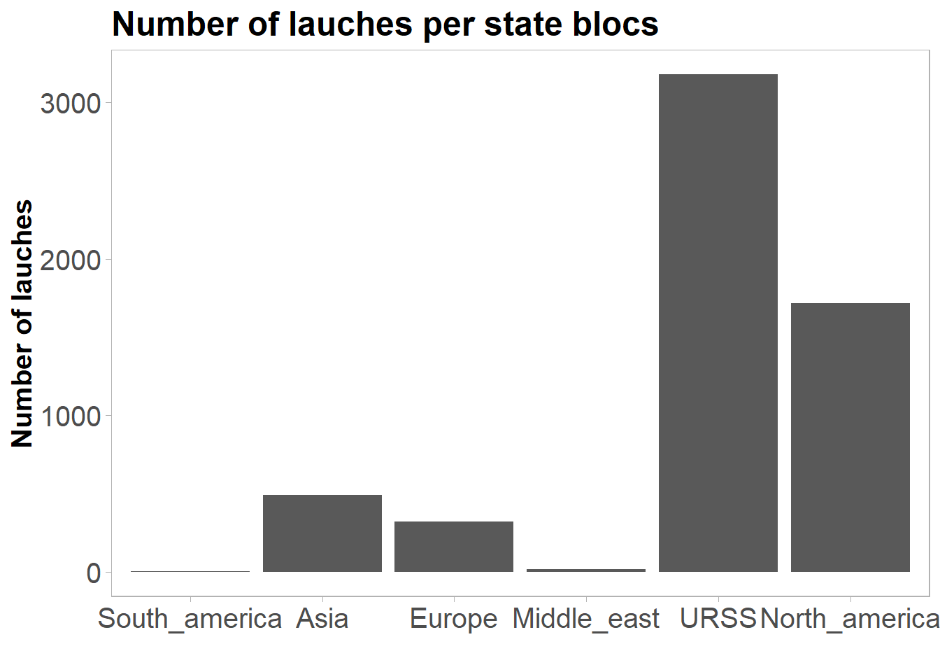
Let’s have a look at the launches across time per country.
launches %>%
  count(launch_year, state_name, state_bloc) %>%
  ggplot(aes(x = launch_year, y = n)) +
  geom_line(size = 2) +
  labs(title = "Number of lauches per state",
       x = "",
       y = "Number of lauches") +
  facet_wrap(~state_bloc, scales = "free") +
  facet_wrap(~state_name) +
  theme(panel.grid = element_blank(),
        strip.text = element_text(face = "bold")) +
   scale_x_continuous("", breaks = seq(1960, 2020, 10)) +
  my_theme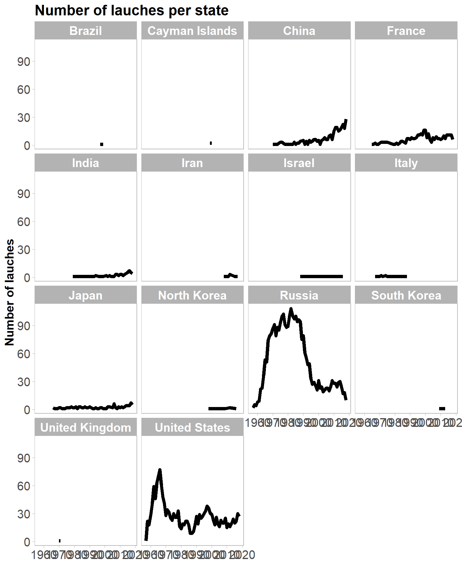
It is not bad, but I will use the shortened list of country as Dave Robinson did to make comparisons between countries easier.
launches %>%
  count(state_name_short, launch_year) %>%
  mutate(state_name_short = fct_reorder(state_name_short, -n, sum)) %>%
  ggplot(aes(x = launch_year, y = n,
             colour = state_name_short)) +
  geom_line(size = 1.5) +
  labs(title = "Number of lauches per state (short list)",
       x = "Year of launch",
       y = "Number of lauches",
       colour = "State") +
  theme_minimal() +
   theme(panel.grid = element_blank(),
        strip.text = element_text(face = "bold")) +
   scale_x_continuous("", breaks = seq(1960, 2020, 10)) +
  my_theme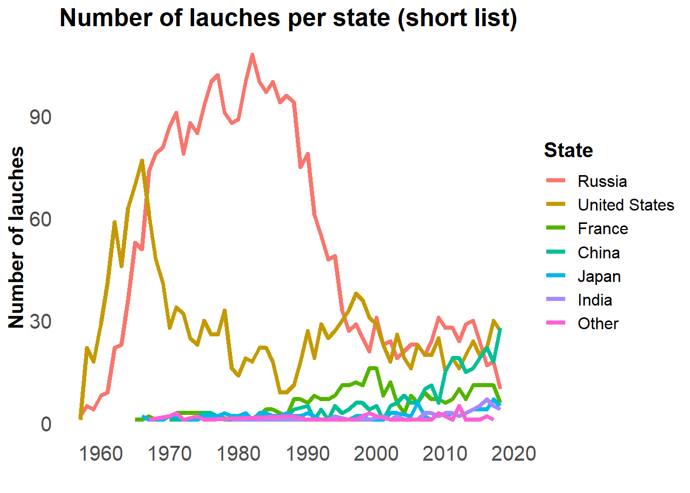
Lets have a look with the geographical blocs.
launches %>%
  count(state_bloc, launch_year) %>%
  mutate(state_bloc = fct_reorder(state_bloc, -n, sum)) %>%
  ggplot(aes(x = launch_year, y = n,
             colour = state_bloc)) +
  geom_line(size = 1.5) +
  labs(title = "Number of lauches per state bloc",
       subtitle = "US and USSR dominated the early race, \nAsia is booming now",
       x = "Year of launch",
       y = "Number of lauches",
       colour = "State bloc") +
  theme_minimal() +
  theme(panel.grid = element_blank()) +
   scale_x_continuous("", breaks = seq(1960, 2020, 10)) +
  my_theme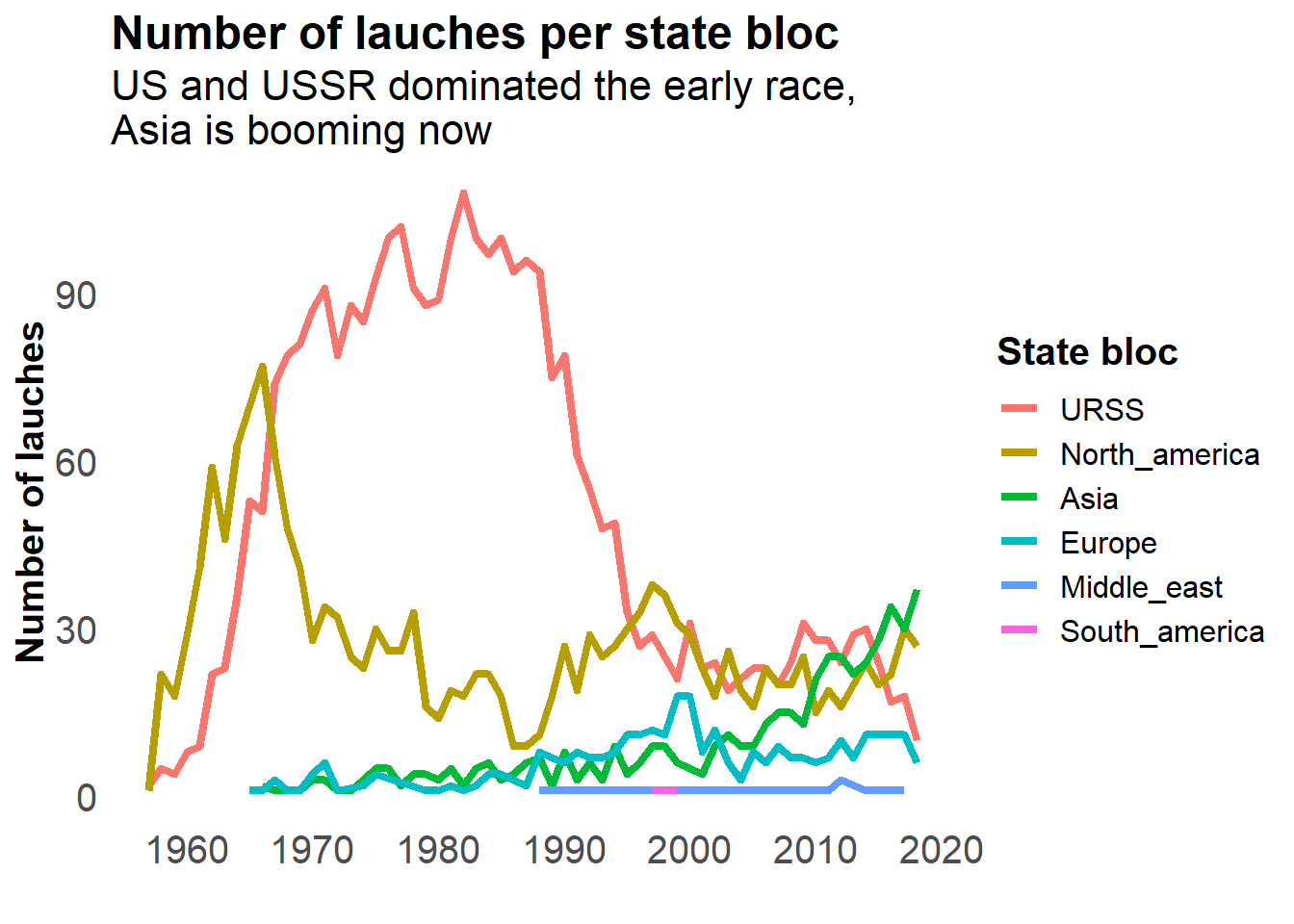
I like how it is shows that Asia has grown so much recently.
The United states began the space race, closely followed by Russia, which dominated the number of launches until the late nineties. After that, Russia and the US were stable and equivalent. In the early 2000, China, followed by India increased their shares of the launches more recently.
US vs Russia
Since for a long time the race was dominated by the US and Russia, let’s compare the two.
launches %>%
  filter(state_name %in% c("United States", "Russia")) %>%
   ggplot(aes(x = launch_year, fill = state_name)) +
  geom_area(stat = "bin",
            position = "identity",
            bins = 30, alpha = 0.6) +
  scale_fill_manual(values = c("#999999", "#E69F00")) +
    theme_minimal() +
  theme(panel.grid = element_blank(),
        strip.text = element_text(face = "bold")) +
  labs(title = "Space race: US vs Russia",
       subtitle = "Numer of launches per year in Russia and \nthe states",
       x = "Year of launches ",
       y = "Number of launches",
       fill = "") +
   scale_x_continuous("", breaks = seq(1960, 2020, 10)) +
  my_theme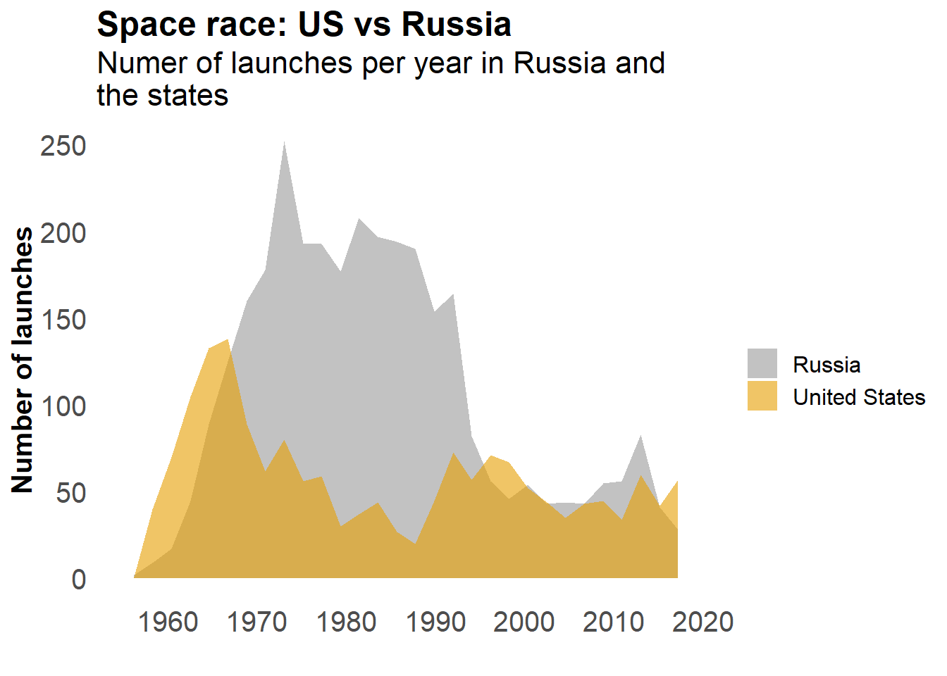
Success vs Failure
We have the information on whether the launch was a success or a failure. Let’s have a look at how the number of failures evolved though time.
launches %>%
  count(category, launch_year) %>%
  ggplot(aes(x = launch_year, y = n,
             fill = category)) +
  geom_bar(stat = "identity",
            #position = "identity",
            ) +
  scale_fill_manual(values = c("#999999", "#E69F00")) +
    theme_minimal() +
  theme(panel.grid = element_blank(),
        strip.text = element_text(face = "bold")) +
  labs(title = "Number of successfull and failed launches accross time",
       subtitle = "It seems the number of failed launches \ndecreases with time",
       x = "Year of launches ",
       y = "Number of launches",
       fill = "Launch outcome") +
  scale_x_continuous("", breaks = seq(1960, 2020, 10)) +
  my_theme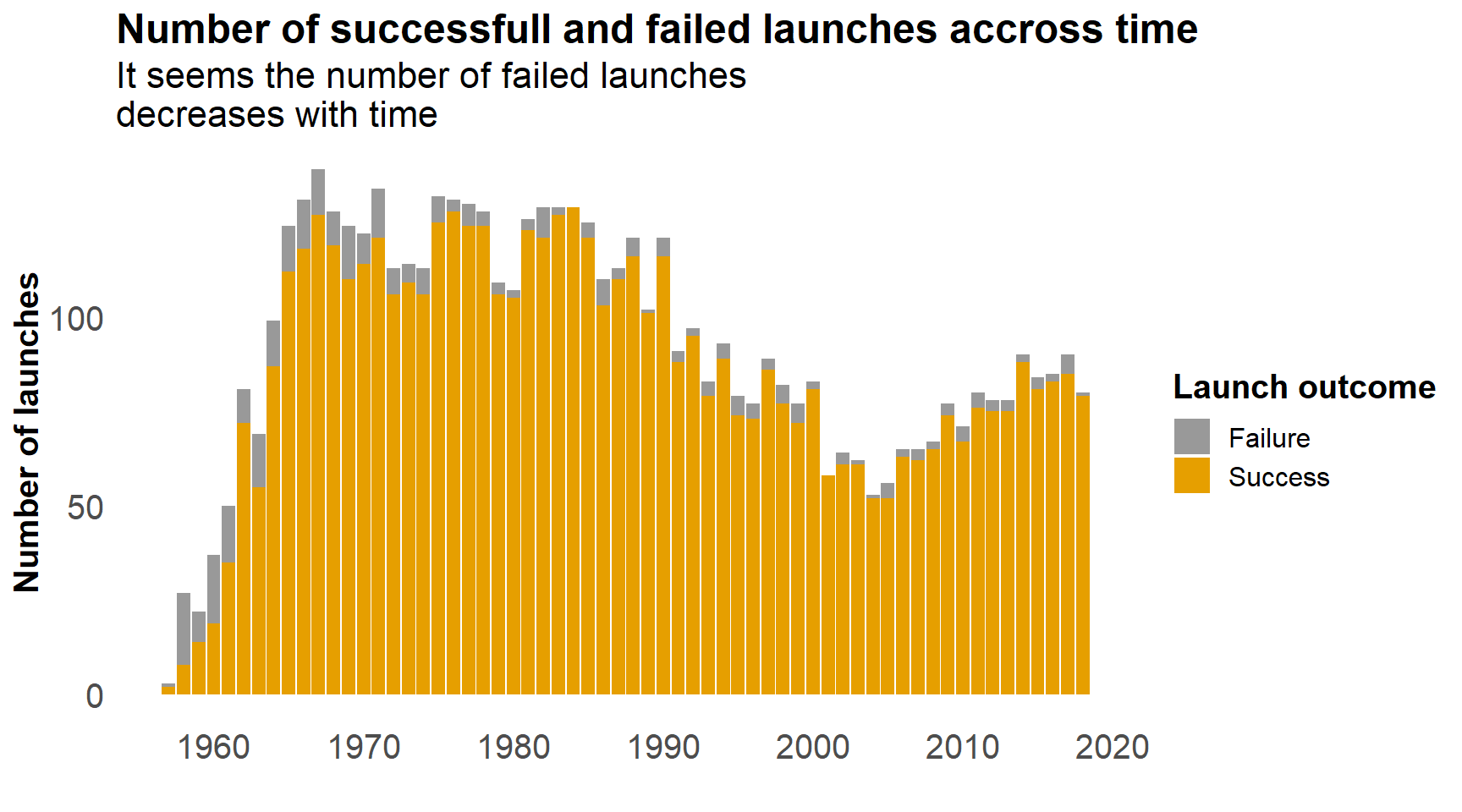
Sweet. Let’s have a look by country, focusing on the countries that send most launches.
launches %>%
  filter(state_name %in% c("China", "France", "Russia", "United States")) %>%
  count(category, launch_year, state_name_short) %>%
  ggplot(aes(x = launch_year, y = n,
             fill = category)) +
  geom_bar(stat = "identity") +
  facet_wrap(~state_name_short, nrow = 4) +
  scale_fill_manual(values = c("#999999", "#E69F00")) +
    theme_minimal() +
  theme(panel.grid = element_blank(),
        strip.text = element_text(face = "bold")) +
  labs(title = "Number of successfull and failed launches accross time",
       subtitle = "Per country",
       x = "Year of launches ",
       y = "Number of launches",
       fill = "Launch outcome") +
  scale_x_continuous("", breaks = seq(1960, 2020, 10)) +
  my_theme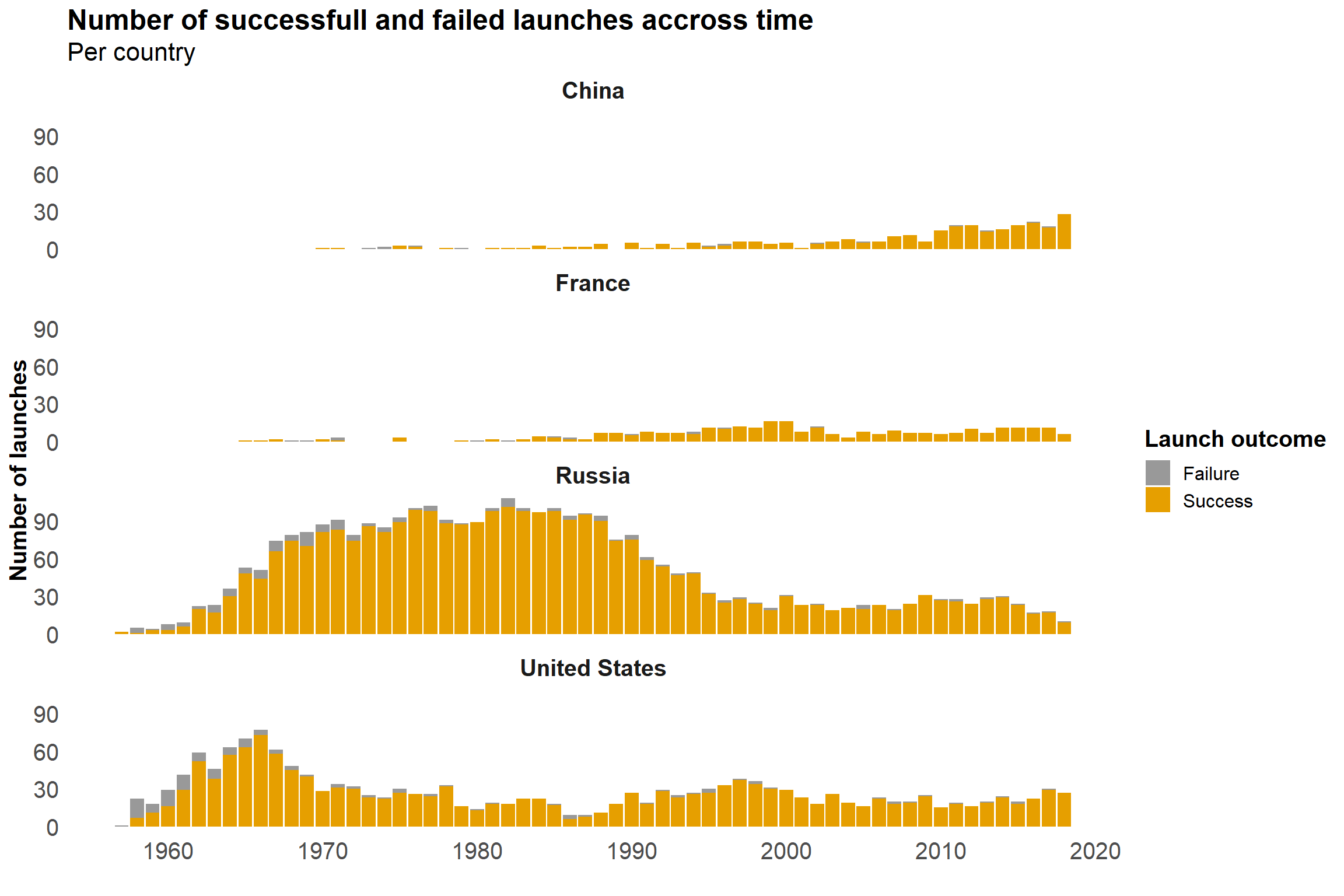
It’s nice, but I would have to have a look at the proportion of failed launches.
launches %>%
  filter(state_name %in% c("China", "France", "Russia", "United States")) %>%
  group_by(state_name, launch_year) %>%
  add_tally() %>%
  add_count(category) %>%
  distinct(state_bloc, launch_year, category, n, nn) %>%
  mutate(proportion = nn / n) %>%
  ggplot(aes(x = launch_year, y = proportion*100,
             fill = category)) +
  geom_bar(stat = "identity") +
  facet_wrap(~state_name, nrow = 4) +
  labs(title = "Space mastery increases with time",
       subtitle = "Countries experienced many failures in their early years. \nNowadays, lauches are mostly successfull",
       x = "Year of launch",
       y = "Percentage of lauches",
       fill = "Launch outcome") +
  scale_fill_manual(values = c("#999999", "#E69F00")) +
    theme_minimal() +
  theme_minimal() +
   theme(panel.grid = element_blank(),
        strip.text = element_text(face = "bold")) +
  scale_x_continuous("", breaks = seq(1960, 2020, 10)) +
  my_theme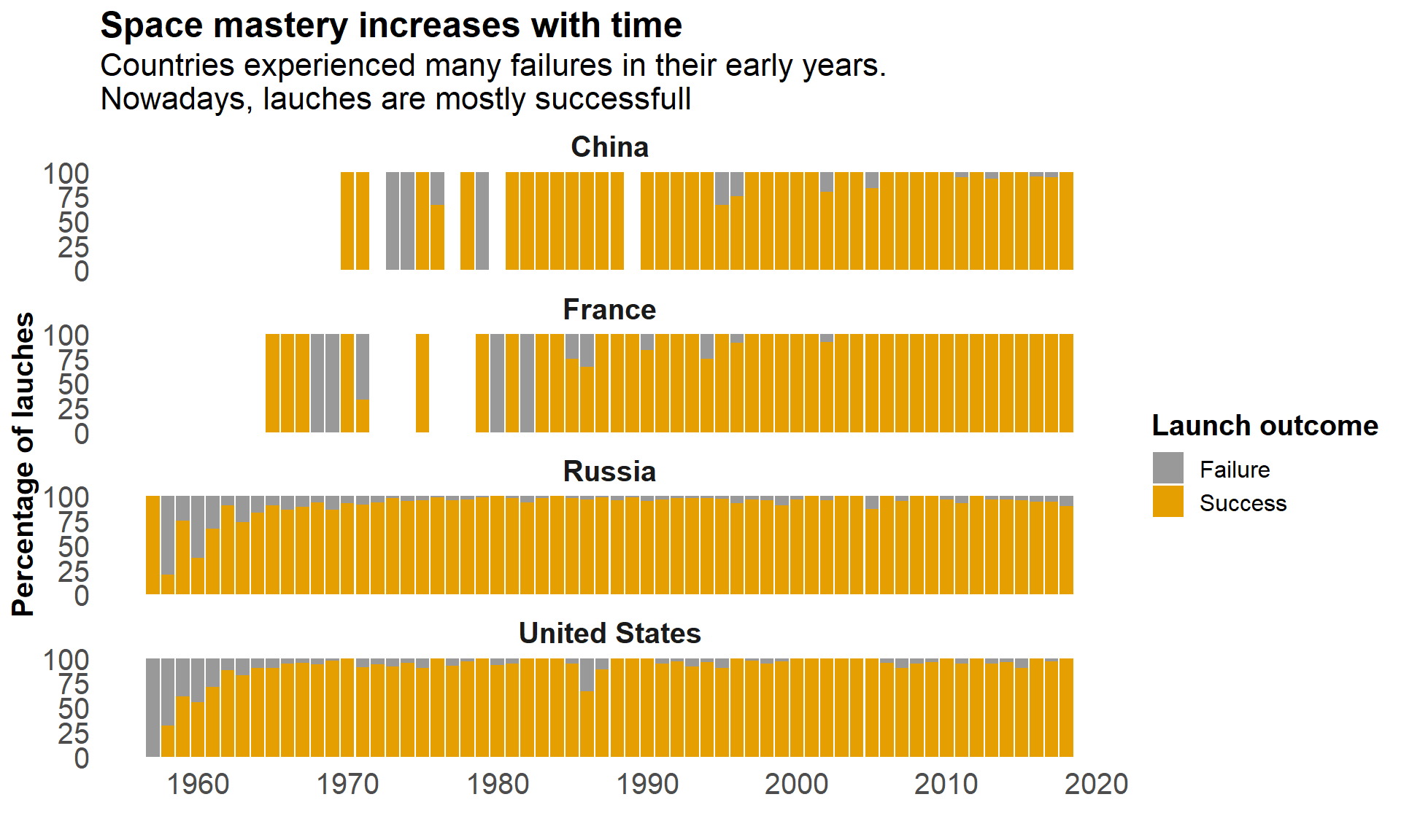
Cool, so everybody improves after some times.
Private vs public lauches
Now I wanted to see whether the launches were mostly made by states or by private companies, and how this varied with time.
launches %>%
  filter(state_bloc != "South_america" & state_bloc != "Middle_east") %>%
  ggplot(aes(x = launch_year, fill = agency_type) ) +
  geom_histogram(bins = 62) +
  facet_wrap(vars(state_bloc), nrow = 4) +
  theme_minimal() +
  theme(panel.grid = element_blank(),
        strip.text = element_text(face = "bold")) +
    scale_fill_brewer(palette = "Set1") +
  labs(title = "Who accounts for space launches in different blocs?",
       subtitle = "While in Europe and in the states the market has been recently privatised, \nstate still accounts for most lauches in Asia and Russia",
       x = "Year of launch",
       y = "Number of launches",
       fill = "Type of agency") +
   scale_x_continuous("", breaks = seq(1960, 2020, 10)) +
  my_theme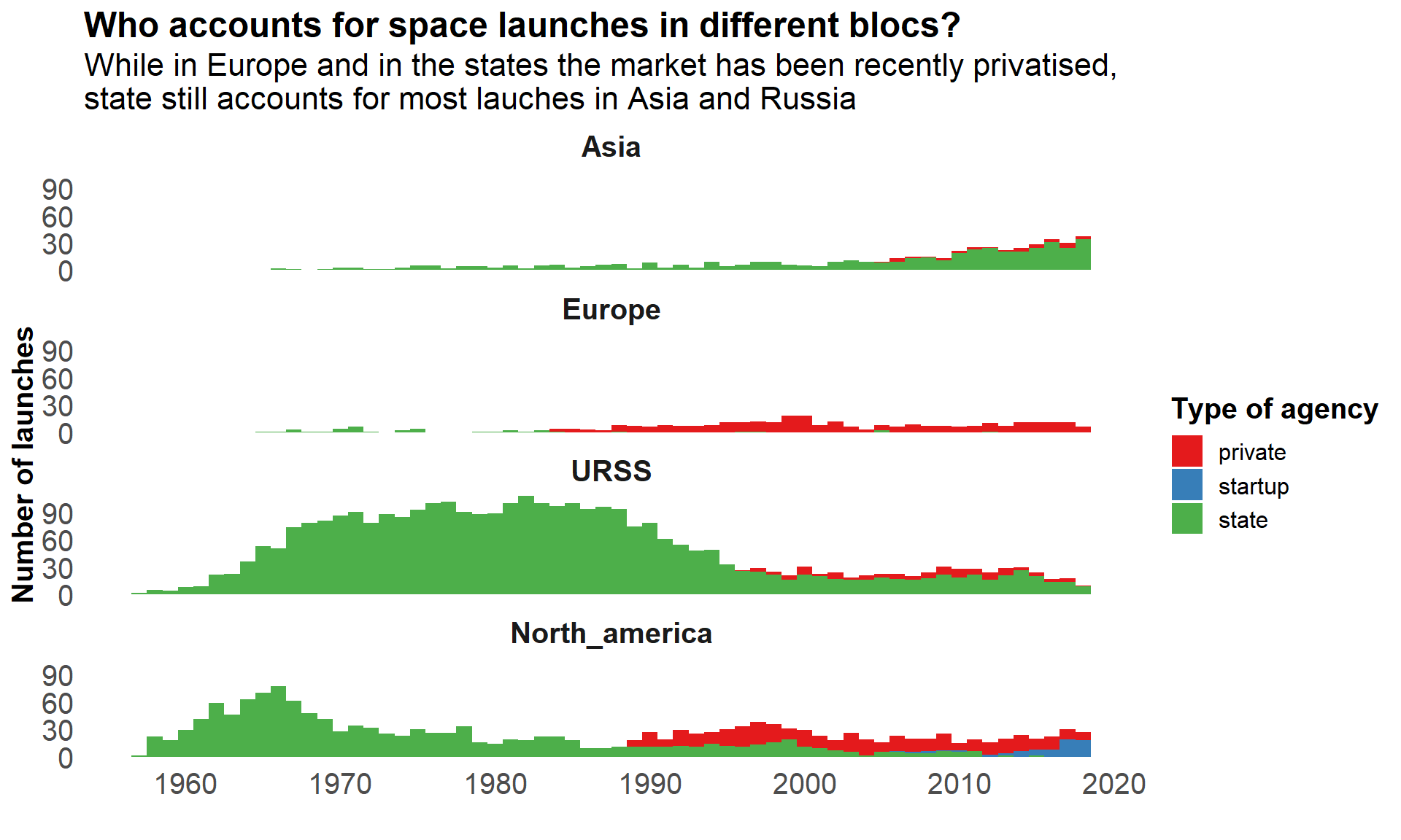
launches %>%
  filter(state_bloc != "South_america" & state_bloc != "Middle_east") %>%
  select(state_bloc, launch_year, agency_type) %>%
  group_by(state_bloc, launch_year) %>%
  add_tally() %>%
  add_count(agency_type) %>%
  distinct(state_bloc, launch_year, agency_type, n, nn) %>%
  mutate(proportion = nn / n) %>%
  ggplot(aes(x = launch_year, y = proportion*100,
             fill = agency_type)) +
  geom_bar(stat = "identity") +
  facet_wrap(~state_bloc, nrow = 4) +
  labs(title = "Number of lauches per state bloc",
       subtitle = "While in Europe and in the states the market has been recently privatised, \nstate still accounts for most lauches in Asia and Russia",
       x = "Year of launch",
       y = "Percentage of lauches",
       fill = "Type of agency") +
  scale_fill_brewer(palette = "Set1") +
  theme_minimal() +
   theme(panel.grid = element_blank(),
        strip.text = element_text(face = "bold")) +
   scale_x_continuous("", breaks = seq(1960, 2020, 10)) +
  my_theme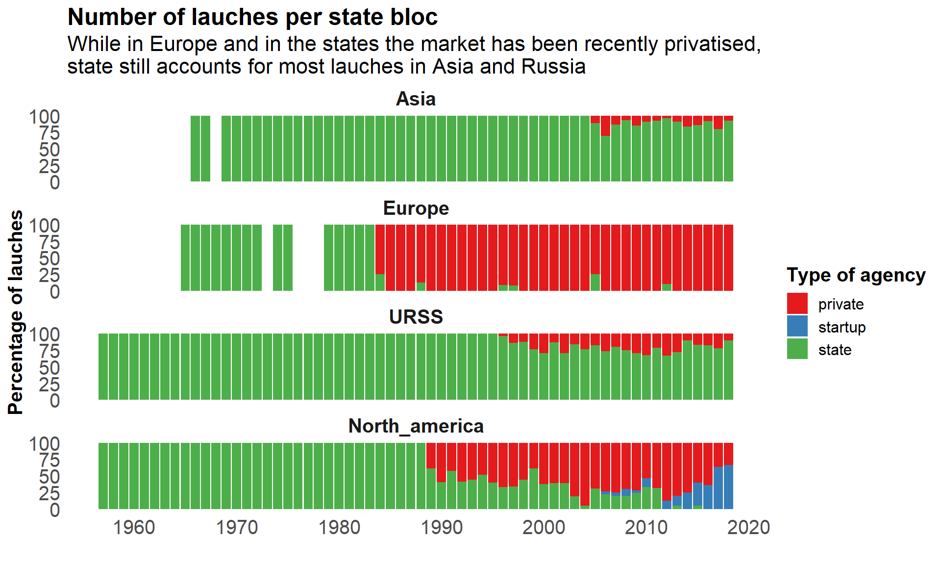
While launches were performed by state agencies for a long time, the private sector operates most of the launches nowadays in Europe and in the States.
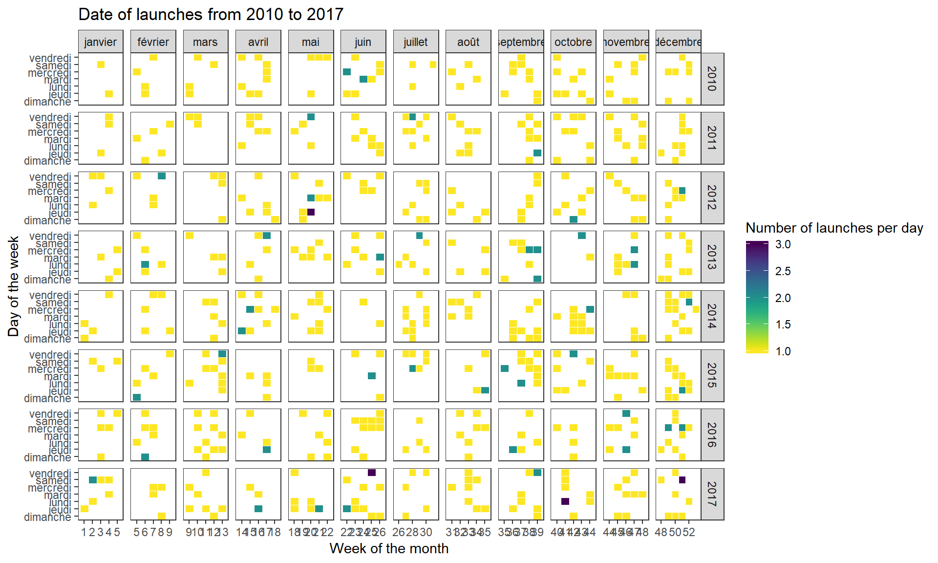
Date of launches
Since the data is so huge, I focus on an early period of the space exploration, and on the past decade.
launches %>%
  drop_na(launch_month, launch_week_num, launch_weekday, launch_year) %>%
  filter(launch_year %in% c(1965:1970)) %>%
  count(launch_year, launch_month,
        launch_weekday, launch_week_num) %>%
  ggplot(aes(x = launch_week_num,
             y = launch_weekday)) +
  geom_tile(aes(fill = n),colour = "white", na.rm = TRUE) +
  facet_grid(vars(launch_year), vars(launch_month),
             scale = "free") +
  scale_fill_viridis(option = "viridis",
                     direction = -1) +
  #scale_fill_gradient(low="red", high="yellow") +
  theme_bw() +
  labs(title = "Date of launches from 1965 to 1970",
       x = "Week of the month",
       y = "Day of the week",
       fill = "Number of launches per day") +
  theme(panel.grid.major = element_blank(),
        panel.grid.minor = element_blank())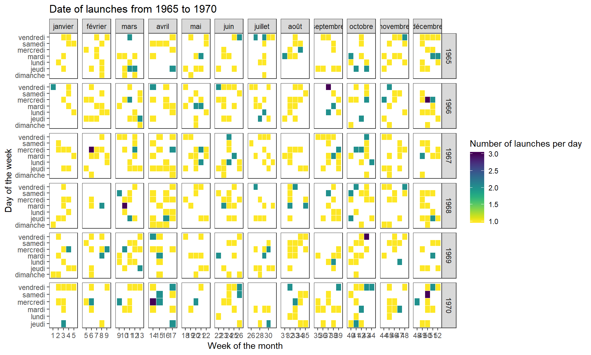
launches %>%
  drop_na(launch_month, launch_week_num, launch_weekday, launch_year) %>%
  filter(launch_year %in% c(2010:2017)) %>%
  count(launch_year, launch_month,
        launch_weekday, launch_week_num) %>%
  ggplot(aes(x = launch_week_num,
             y = launch_weekday)) +
  geom_tile(aes(fill = n),colour = "white", na.rm = TRUE) +
  facet_grid(vars(launch_year), vars(launch_month),
             scale = "free") +
  scale_fill_viridis(option = "viridis",
                     direction = -1) +
  theme_bw() +
  labs(title = "Date of launches from 2010 to 2017",
       x = "Week of the month",
       y = "Day of the week",
       fill = "Number of launches per day") +
  theme(panel.grid.major = element_blank(),
        panel.grid.minor = element_blank())