I will use the #Tidytuesday data on U.S. R&D funding to perform a simple cluster analysis in R. Since I never performed such an analysis in R, I followed and somewhat modified the code written by Otho Mantegazza.

For details on the data set, see the previous post.

First we import the data directly from Github.

feder_spendings <- read.csv("https://raw.githubusercontent.com/rfordatascience/tidytuesday/master/data/2019/2019-02-12/fed_r_d_spending.csv")

The dataset is relatively simple. Here we are interested in the funding spent by the U.S. government to each of the federal agencies for R&D over the years.

Correlation in funding over time

We saw in the previous post that the temporal evolution of funding varies between agencies over time. We would like to better understand which agencies share similar trends in funding over time.

First easy approach: correlations.

The base R cor() function need the data in columns, that is, in a wide format. We use spread() from tidyr to transform the dataframe from long to wide.

feder_spendings_wide <- feder_spendings %>% 
  select(department, year, rd_budget) %>% 
  spread(key   = department,
         value = rd_budget)

Correlation matrix

feder_spendings_wide %>% 
  column_to_rownames("year") %>%
  cor() %>% 
  round(2) %>% 
  kable()

	DHS	DOC	DOD	DOE	DOT	EPA	HHS	Interior	NASA	NIH	NSF	Other	USDA	VA
DHS	1.00	0.50	0.78	0.02	0.22	-0.34	0.86	-0.36	0.15	0.86	0.80	-0.24	0.76	0.74
DOC	0.50	1.00	0.36	-0.17	0.33	-0.11	0.78	-0.14	0.55	0.77	0.78	-0.16	0.74	0.77
DOD	0.78	0.36	1.00	-0.28	-0.07	-0.51	0.77	-0.61	-0.08	0.78	0.73	-0.38	0.73	0.61
DOE	0.02	-0.17	-0.28	1.00	0.27	0.05	-0.11	0.57	0.01	-0.12	0.00	0.53	-0.16	-0.01
DOT	0.22	0.33	-0.07	0.27	1.00	0.31	0.23	0.38	0.29	0.22	0.22	-0.05	0.25	0.25
EPA	-0.34	-0.11	-0.51	0.05	0.31	1.00	-0.35	0.52	0.52	-0.36	-0.46	0.15	-0.21	-0.38
HHS	0.86	0.78	0.77	-0.11	0.23	-0.35	1.00	-0.38	0.32	1.00	0.96	-0.28	0.92	0.93
Interior	-0.36	-0.14	-0.61	0.57	0.38	0.52	-0.38	1.00	0.39	-0.40	-0.32	0.52	-0.33	-0.36
NASA	0.15	0.55	-0.08	0.01	0.29	0.52	0.32	0.39	1.00	0.31	0.24	0.23	0.40	0.23
NIH	0.86	0.77	0.78	-0.12	0.22	-0.36	1.00	-0.40	0.31	1.00	0.96	-0.29	0.92	0.93
NSF	0.80	0.78	0.73	0.00	0.22	-0.46	0.96	-0.32	0.24	0.96	1.00	-0.23	0.82	0.95
Other	-0.24	-0.16	-0.38	0.53	-0.05	0.15	-0.28	0.52	0.23	-0.29	-0.23	1.00	-0.26	-0.27
USDA	0.76	0.74	0.73	-0.16	0.25	-0.21	0.92	-0.33	0.40	0.92	0.82	-0.26	1.00	0.78
VA	0.74	0.77	0.61	-0.01	0.25	-0.38	0.93	-0.36	0.23	0.93	0.95	-0.27	0.78	1.00

It’s a bit difficult to see the patterns so let’s get a nice graphic visualization.

I use the ggally packages, which draws nice heatmaps out of a correlation matrix for us. To do this without the aid of yet another helper package, see Otho’s code

the ggcorr() function also take data with variables to correlate stored in columns, like the base R function.

ggcorr(feder_spendings_wide,
       label = TRUE,
       nbreaks = 7,
       palette = "RdBu")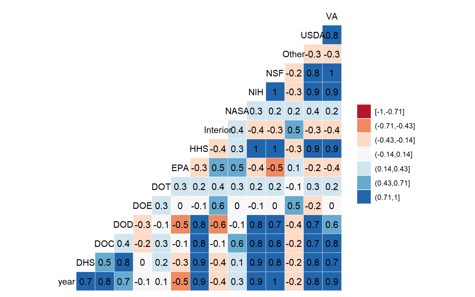

There are groups of agencies whose funding with time seem to be quite correlated (for example: DOD, NIH, NSF, HHS). To further explore the similarities of the evolution of funding between agencies, let’s make a little cluster analysis.

Cluster analysis

In a cluster analysis, we try to create clusters of agencies where funding is similar within cluster, and dissimilar between clusters.

We are going to use an agglomerative type of clustering: we begin with observations, we combine the more similar in clusters, and then we merge clusters that are similar until we are satisfied. It is a bottom-up approach.

There are many way to measure the similarity between observations or clusters. Here we will use the euclidian distance as a metric, which is a reasonable choice for continuous numerical values.

Scaling

Since there is a huge variation in the magnitude of the budget received by the agencies, we cannot perform the clustering on the raw data, We want the similarities in the temporal evolution of funding, so we need to scale/normalize the data.

A pretty common scaling is made by substracting the mean and dividing by the standard deviation or the variance. However, this leads to negative values of funding, which is not very nice. Otho decided to scale the data between 0 and 1, and I follow his lead. To do that, we use the rescale() function from the scale package that we used in the previous post.

This is also a nice example of how to use the mutate_at() from the dplyr package, which allows automatic selection of column on which to apply a function. Here we select columns whose title countain “year”.

# scale each variable between 0 and 1
feder_wide_01 <- 
  feder_spendings_wide %>%
  mutate_at(vars(-contains("year")),
            ~scales::rescale(., to = c(0,1),
                             from = c(0, max(.))))


# this is how it looks after scaling and rounding
feder_wide_01 %>% 
  head() %>% 
  round(2) %>% 
  kable()

year	DOC	DOD	DOE	DOT	EPA	HHS	Interior	NASA	NIH	NSF	Other	USDA	VA
1976	0.45	0.38	0.69	0.94	0.82	0.25	0.98	0.85	0.23	0.38	0.48	0.59	0.30
1977	0.46	0.40	0.88	0.90	0.82	0.26	0.92	0.86	0.23	0.38	0.52	0.58	0.27
1978	0.48	0.39	1.00	0.95	1.00	0.28	0.96	0.85	0.25	0.39	0.50	0.63	0.26
1979	0.52	0.39	1.00	0.82	0.94	0.27	1.00	0.89	0.26	0.38	0.94	0.66	0.26
1980	0.52	0.39	0.97	0.86	0.77	0.27	0.92	0.94	0.26	0.38	1.00	0.61	0.26
1981	0.45	0.44	0.94	0.80	0.77	0.26	0.84	0.90	0.24	0.37	0.78	0.63	0.28

To perform the hierarchical clustering, we need to transpose the data, because the hcclust() function clusters the rows, not the columns of a data frame.

rd_for_clust <- feder_wide_01 %>%
  column_to_rownames("year") %>%
  t()

Now we take the Euclidean distance, and we do the hierarchical clustering.

rd_hclust <- rd_for_clust %>% 
  dist() %>%  # Euclidean distance
  hclust()    # hierarchical cluster on dissimilarity

Now we visualize.

rd_hclust %>% plot()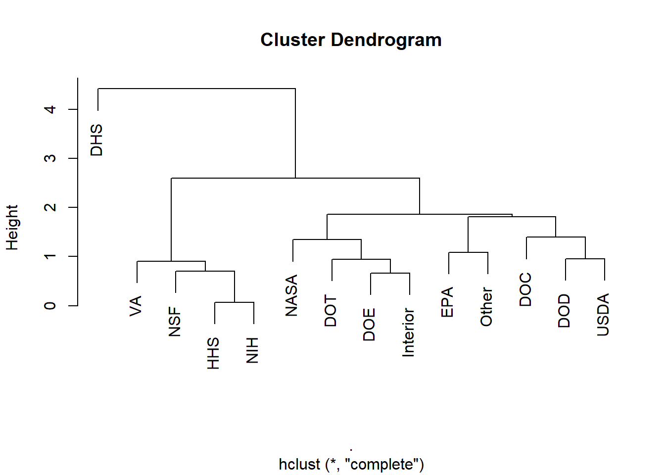

We can have a nicer plt with the superheat() function from the superheat package.

rd_for_clust %>% 
  superheat::superheat(row.dendrogram = TRUE,
                       left.label.text.size = 5,
                       left.label.text.alignment = "center",
                       
                       bottom.label.text.angle = 90,
                       bottom.label.text.size = 5,
                       
                       grid.hline.col = "grey40",
                       grid.vline.col = "grey40",
                       
                       title      = "U.S. R&D funding",
                       title.size = 8,
                       
                       row.title      = "Federal agencies",
                       row.title.size = 6,
                       
                       column.title   = "Year",
                       column.title.size = 6)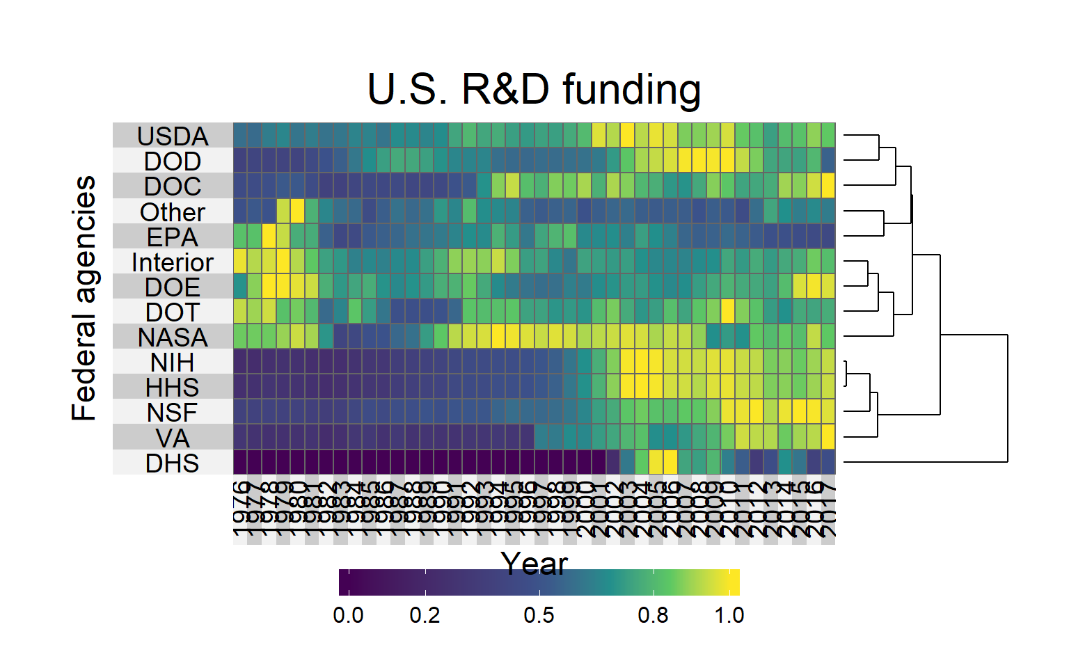

The DHS (Department of Homeland Security) is the most outer group, which is probably because the agency was established in the way it is now in 2001 (after the 11 September terrorist attacks).
VA, HHS, NIH and HHS cluster together, with an increase of funding in the 2000’s, but very low funding before.
USDA, DOD ans DOC also have higher funding recently, but more in the early 2000’s than now.
EPA and Others cluster together, a very early peak of funding, and then very low and decreasing funding.
Interior, DOE, DOT and NASA are in the same group, which is the “heterogeneous group”, with funding increasing and decreasing at various moments.

#Tidytuesday 7: U.S. R&D Budget (part 2): hierarchical clustering

Correlation in funding over time

Cluster analysis

Scaling