Last take on the High Speed French Train delays. Thanks to my slightly obsessive posting of delay graphs on Twitter, Thomas Mock suggested submitting the data to the #Tidytuesday challenge. So did I, and now everybody is plotting graphs of French trains delays. It is so cool to see what other people did! I will probably make a best-of of what I really liked some day.
Originally, when I downloaded the files from SNCF website for the first time, my aim was to map stations and plot their delays. However, things did not go as planned. This is what I wrote in the last post.
Originally, for this post, I wanted to map the data on a French map, but I encountered a bit of trouble in getting the GPS coordinates of the stations, and I am still perfecting my fuzzyjoining. This might be a story for later, including the crushing of my cute naivety concerning name harmonizing in datasets made available within the same company.
Today is the story of my crushed naivety, in the Part 1. Be ready for complaining, frustration, and no fairy-tale ending. I am mostly documenting it as a double reminder to myself: i) how to do fuzzy-joining and ii) why consistency in names is important, and ID columns should not be messed with!
I however won’t admit defeat that easily. I am a scientist, and I have spent months counting thousands of seeds, one month figuring out the perfect timing for pollinating a small Brassicaceae that you never heard of (it’s a cool plant, though), weeks weighing plant bits and dissecting pollen anthesis under the binocular. You don’t get me to quit that easily.
One day, in the middle of the night, I remembered that I saw the number of people going through stations somewhere. I decided to have another go at mapping SNCF stations. This is the Part 2. Nothing too fancy, but we get to make some maps, eventually!
Part 1: on the path to the dirty data hell circles
We import a bunch of data files from the SNCF website.
# Import data
tgv <- read_delim("2019-02-08-regularite-mensuelle-tgv-aqst.csv",
                  ";", escape_double = FALSE, trim_ws = TRUE)
## Parsed with column specification:
## cols(
## .default = col_double(),
## service = col_character(),
## departure_station = col_character(),
## arrival_station = col_character(),
## cancelation_comment = col_logical(),
## comment_delay_departure = col_logical(),
## comment_delay_arrival = col_character(),
## year_month = col_character()
## )## See spec(...) for full column specifications.european_stations <- read_delim("2019-03-01-european-train-stations.csv",
";", escape_double = FALSE, trim_ws = TRUE)## Parsed with column specification:
## cols(
## .default = col_character(),
## id = col_double(),
## uic = col_double(),
## uic8_sncf = col_double(),
## parent_station_id = col_double(),
## is_city = col_logical(),
## is_main_station = col_logical(),
## is_suggestable = col_logical(),
## sncf_is_enabled = col_logical(),
## idtgv_is_enabled = col_logical(),
## db_id = col_double(),
## db_is_enabled = col_logical(),
## busbud_is_enabled = col_logical(),
## ouigo_is_enabled = col_logical(),
## trenitalia_id = col_double(),
## trenitalia_is_enabled = col_logical(),
## ntv_rtiv_id = col_logical(),
## ntv_is_enabled = col_logical(),
## hkx_id = col_logical(),
## hkx_is_enabled = col_logical(),
## renfe_id = col_double()
## # ... with 5 more columns
## )
## See spec(...) for full column specifications.## Warning: 35 parsing failures.
## row col expected actual file
## 2939 hkx_id 1/0/T/F/TRUE/FALSE 108000044 '2019-03-01-european-train-stations.csv'
## 4090 ntv_rtiv_id 1/0/T/F/TRUE/FALSE 1325 '2019-03-01-european-train-stations.csv'
## 5006 hkx_id 1/0/T/F/TRUE/FALSE 108000105 '2019-03-01-european-train-stations.csv'
## 5313 ntv_rtiv_id 1/0/T/F/TRUE/FALSE 3009 '2019-03-01-european-train-stations.csv'
## 5658 ntv_rtiv_id 1/0/T/F/TRUE/FALSE 2617 '2019-03-01-european-train-stations.csv'
## .... ........... .................. ......... ........................................
## See problems(...) for more details.gares <- read_delim("2019-03-01-referentiel-gares-voyageurs.csv",
";", escape_double = FALSE, trim_ws = TRUE)## Parsed with column specification:
## cols(
## .default = col_character(),
## `Nbre plateformes` = col_double(),
## `Code postal` = col_double(),
## `Code commune` = col_double(),
## `Code département` = col_double(),
## `Longitude WGS84` = col_double(),
## `Latitude WGS84` = col_double(),
## `Code UIC` = col_double(),
## `Niveau de service` = col_double(),
## SOP = col_logical(),
## `Date fin validité plateforme` = col_date(format = "")
## )
## See spec(...) for full column specifications.These data are from the Open Data from the SNCF website, and you can also find them on the #Tidytuesday website.
Outer hell circle: stations
So here are the train stations in the dataset:
tgv$arrival_station %>% unique()## [1] "METZ" "PARIS EST"
## [3] "STRASBOURG" "AVIGNON TGV"
## [5] "BELLEGARDE (AIN)" "BESANCON FRANCHE COMTE TGV"
## [7] "PARIS LYON" "GRENOBLE"
## [9] "MACON LOCHE" "MARSEILLE ST CHARLES"
## [11] "MULHOUSE VILLE" "ANGERS SAINT LAUD"
## [13] "PARIS MONTPARNASSE" "POITIERS"
## [15] "RENNES" "FRANCFORT"
## [17] "LAUSANNE" "PARIS NORD"
## [19] "LILLE" "NANCY"
## [21] "LE CREUSOT MONTCEAU MONTCHANIN" "NICE VILLE"
## [23] "ZURICH" "NANTES"
## [25] "VANNES" "DOUAI"
## [27] "DUNKERQUE" "LYON PART DIEU"
## [29] "DIJON VILLE" "PERPIGNAN"
## [31] "TOULOUSE MATABIAU" "ARRAS"
## [33] "REIMS" "NIMES"
## [35] "TOULON" "BORDEAUX ST JEAN"
## [37] "LE MANS" "STUTTGART"
## [39] "GENEVE" "ANGOULEME"
## [41] "VALENCE ALIXAN TGV" "ITALIE"
## [43] "MONTPELLIER" "ST MALO"
## [45] "BREST" "LA ROCHELLE VILLE"
## [47] "AIX EN PROVENCE TGV" "LAVAL"
## [49] "QUIMPER" "ANNECY"
## [51] "CHAMBERY CHALLES LES EAUX" "ST PIERRE DES CORPS"
## [53] "SAINT ETIENNE CHATEAUCREUX" "TOURS"
## [55] "TOURCOING" "BARCELONA"
## [57] "PARIS VAUGIRARD" "MARNE LA VALLEE"
## [59] "MADRID"There is a mix of French and European stations. I would like to plot them on a map of Europe, so I need to fetch their GPS coordinates.
I found a data file from Trainline, a train travel agent, with the location of all the stations that are in their database. As they sell French train tickets, the stations in the SNCF dataset should be referenced in their database. I just have to join them.
Some text cleaning first: I use the str_to_title() function from stringr to change all caps to title caps.
tgv <- tgv %>%
  mutate(arrival_station = str_to_title(arrival_station),
         departure_station = str_to_title(departure_station))
Second hell inner circle: joining
Ok, let’s see which stations will not get coordinates.
anti_join(tgv, european_stations, by = c("arrival_station" = "name")) %>% nrow()## [1] 3046Like… a lot. How is that so? Let’s have a look at Paris stations.
tgv %>%
  select(arrival_station) %>%
  filter(str_detect(arrival_station, "Paris")) %>%
  distinct()
## # A tibble: 5 x 1
## arrival_station
## <chr>
## 1 Paris Est
## 2 Paris Lyon
## 3 Paris Montparnasse
## 4 Paris Nord
## 5 Paris Vaugirardeuropean_stations %>%
select(name) %>%
filter(str_detect(name, "Paris")) %>%
distinct()## # A tibble: 39 x 1
## name
## <chr>
## 1 Paris Gare de Lyon RER
## 2 Atlb Paris Nord
## 3 Paris Pereire Saussure
## 4 Paris Ampère Wagram
## 5 Paris Bercy Commercial
## 6 Paris Gare du Nord
## 7 Paris Montparnasse 3 Vaugirard
## 8 Paris Tolbiac TAA
## 9 Paris Section urbaine
## 10 Paris Gare de Lyon A
## # ... with 29 more rowsBecause the names are completely different, that’s why!

Time for Plan B.
I can see that the trainline file has uic, uic8_sncf and sncf_id columns. Which means that somewhere in the SNCF 300 open datasets, there must be a list of stations with their UIC1 code and/or some SNCF ID. It has to!
Some internet searching later…
There is a file that seems to be the station database of SNCF. With all the crunchy little details such as the town, the department, the name of the station as it is written on the building, the number of platforms and, conveniently, longitude and latitude.
Perfect.
To get a feel of how nice things are going to be, let’s check the Paris station names again.
gares %>%
  select(`Intitulé gare`) %>%
  filter(str_detect(`Intitulé gare`, "Paris")) %>%
  distinct()
## # A tibble: 14 x 1
## `Intitulé gare`
## <chr>
## 1 Paris Montparnasse Hall 1 & 2
## 2 Paris Gare du Nord
## 3 Paris Saint-Lazare
## 4 Paris Austerlitz Souterrain
## 5 Paris Austerlitz
## 6 Paris Montparnasse Vaugirard
## 7 Cormeilles-en-Parisis
## 8 Paris Gare du Nord Souterrain
## 9 Paris Gare du Nord transmanche
## 10 Paris Est
## 11 Paris Bercy Bourgogne - Pays d'Auvergne
## 12 Paris Gare du Nord Surface Banlieue
## 13 Paris Gare de Lyon Hall 1 & 2
## 14 Paris Gare de Lyon SouterrainThat… what… how… je ne sais que dire…
I am unpleasantly surprised by some of what I read, to say the least.
For example, we have “Paris Est” (not “Paris Gare de l’Est”) and “Paris Gare du Nord…” (not “Paris Nord”). Why mixing the short and long names?
Other example, “Paris Gare de Lyon Souterrain”" and “Paris Gare de Lyon Hall 1 & 2”" are counted as different stations. Souterrain means “underground”, if you need to know. And I may be wrong but I think that in the station, it’s actually called “Hall 3”.
Obviously, the SNCF did not harmonize its station names across its own files. I am sure there is a special hell for the kind of people who would do that.

Plan C: time to use some fuzzy joining, then.
First hell inner circle: fuzzyjoining
I have to be honest, I never tried fuzzy-joining anything before. I just read the name somewhere on Stackoverflow one day, and filled it for later use. Thank you brain.
The fuzzyjoin package is written by David Robinson and it helps joining columns where the text is not exactly the same, that is, inexact matching.
I believe that it is targeted at text where there are some mistakes and small variations. Some of the names here differ by two or more words, so I am not completely sure of what would happen.
There are several columns that could be of use: RG or UT. I have no idea what the names mean, because apparently data dictionnaries are for loosers .
Some tidying first. I first remove the “GARE” for UT and RG because the word itself in not in the name of the stations in the other file. Then, I harmonize the St/Saint abbreviation problem. And if there are duplicates, I select one of them.
essai_gare <- gares %>%
  drop_na(`Latitude WGS84`, `Longitude WGS84`) %>%
  mutate(intitule_plateforme = str_remove(`Intitulé plateforme`, "Gare de|Gare du"),
         RG = str_to_title(str_remove(RG, "GARE")),
         UT = str_to_title(str_remove(UT, "GARE"))) %>%
  select(name = "Intitulé gare",
         intitule_plateforme,
         RG,
         UT) %>%
  filter(!(name %in% c("Toul", "Die", "Montchanin", "Crest"))) %>%
  mutate(RG = str_replace(RG, " St ", " Saint "),
         UT = str_replace(UT, " St ", " Saint "),
         UT = str_replace(UT, "St ", "Saint "),
         UT = str_remove(UT, "^ P$")) %>%
  group_by(UT) %>% slice(1) %>% ungroup()
Now, I prepare the tgv file.
essai_tgv <- tgv %>%
  select(departure_station) %>%
  unique() %>%
  mutate(departure_station = str_replace(departure_station, " St ", " Saint "),
         departure_station = str_replace(departure_station, "St ", "Saint "))
And let’s go!

fuzzy_left_join(essai_tgv,
                essai_gare,
                by = c("departure_station" = "UT"),
                match_fun = str_detect) %>%
  head(10)
## # A tibble: 10 x 5
## departure_station name intitule_plateforme RG UT
## <chr> <chr> <chr> <chr> <chr>
## 1 Paris Est <NA> <NA> <NA> <NA>
## 2 Reims <NA> <NA> <NA> <NA>
## 3 Paris Lyon <NA> <NA> <NA> <NA>
## 4 Chambery Challes Les Eaux <NA> <NA> <NA> <NA>
## 5 Lyon Part Dieu <NA> <NA> <NA> <NA>
## 6 Montpellier <NA> <NA> <NA> <NA>
## 7 Mulhouse Ville <NA> <NA> <NA> <NA>
## 8 Paris Montparnasse <NA> <NA> <NA> <NA>
## 9 Bordeaux Saint Jean <NA> <NA> <NA> <NA>
## 10 La Rochelle Ville <NA> <NA> <NA> <NA>It did not work well (you can print the whole table, 6 lines were joined).
By looking at the names in the essai_gare, I noticed some weird spaces. We remove them.
essai_gare <- select(essai_gare,
                     name_departure = UT) %>%
  mutate(name_departure = str_trim(name_departure)) %>%
  na.omit()
And try again.
fuzzy_left_join(essai_tgv,
                essai_gare,
                by = c("departure_station" = "name_departure"),
                match_fun = str_detect) %>%
  filter(is.na(name_departure))
## # A tibble: 23 x 2
## departure_station name_departure
## <chr> <chr>
## 1 Lyon Part Dieu <NA>
## 2 Mulhouse Ville <NA>
## 3 Paris Montparnasse <NA>
## 4 Lille <NA>
## 5 Nancy <NA>
## 6 Rennes <NA>
## 7 Nantes <NA>
## 8 Zurich <NA>
## 9 Metz <NA>
## 10 Italie <NA>
## # ... with 13 more rowsIt is a bit better, I get 23 empty lines. Actually, a bit more because I now have some duplicates (Avignon, for example, because the Avignon station gets two matches from the right hand file, so it doubles its lines).
Let’s try with the other fuzzy join function, which uses a distance to match elements. I am afraid it will yield many false positive, but let’s try.
stringdist_left_join(essai_tgv,
                     essai_gare,
                     by = c("departure_station" = "name_departure"),
                     max_dist = 1,
                     ignore_case = FALSE) %>%
  select(departure_station, name_departure) %>%  filter(is.na(name_departure))
## # A tibble: 24 x 2
## departure_station name_departure
## <chr> <chr>
## 1 Lyon Part Dieu <NA>
## 2 Mulhouse Ville <NA>
## 3 Paris Montparnasse <NA>
## 4 Macon Loche <NA>
## 5 Nancy <NA>
## 6 Rennes <NA>
## 7 Valence Alixan Tgv <NA>
## 8 Zurich <NA>
## 9 Metz <NA>
## 10 Italie <NA>
## # ... with 14 more rows24 non-matched lines and many wrong matches. There are probably ways to tweak the distance parameter to decrease these false positive, but I figured the other function is better suited.
Except that then I spent a couple of more hours trying to get the fuzzy join to go further and I did not manage. I tried the other promising column too, to no end.
At some point, I decided that I had lost enough hours of my life attempting to join SNCF files, and that I should move on. I forbade myself to touch this script ever again, except to turn it into a bitter rant about messy data on the internet.
I now feel less lonely in this failure when I read that many people renounced joining the files during the #Tidytuesday challenge. I would be happy to know who managed, and how.
Closing thoughts on that hell
After giving some thinking to it while showering, I figured that I could do several joins, and reduce the right-hand side file little by little. The idea would be something like:
Do the first fuzzy join. Get the lines that did not get a match from the left-hand-side (LHS).
For the case where the failure happen because of the “Ville”/“TGV” problem, make two joins, one with the names that have “Ville” inside, and one with the names that have “TGV” inside.
Get the rest. Try to remove duplicates from the RHS file, be either trimming the last(s) word(s).
Do several loops of the last one.
I think I could probably manage to get something. But it is an incredible dirty and painful way of doing it. I decided that I had more interesting things to do with my life than compensating for dubious data-management on my free time2.
I made my peace with not plotting anything related to SNCF on maps.
SNCF mapping, the retour!
But then was I thinking of my future while shaving3 when I remembered seeing the number of passengers going through stations somewhere on the SNCF Open data website. And that is cool data to plot on a map.
So mapping SNCF data, take 2!
library(janitor)## Warning: le package 'janitor' a été compilé avec la version R 3.5.2library(hrbrthemes)
library(sf)## Warning: le package 'sf' a été compilé avec la version R 3.5.2## Linking to GEOS 3.6.1, GDAL 2.2.3, PROJ 4.9.3library(tmap)## Warning: le package 'tmap' a été compilé avec la version R 3.5.2library(leaflet)## Warning: le package 'leaflet' a été compilé avec la version R 3.5.2library(ggrepel)## Warning: le package 'ggrepel' a été compilé avec la version R 3.5.2I found a “station list” file, which is not the “reference list of stations” file that we have attempted to put to use before. It contains the Lambert coordinates of all stations, so that’s sweet4. We will let the station reference file sulk on its own in the directory forever, and use the station list file from now on.
For the mapping, I will heavily rely on the advice from Sébastien Rochette.
We will use the sf package (for simple features), whose syntax is inspired from PostGIS. It is a relatively new package in R, but it is quite powerful and quite handy. It enables us to manipulate sf objects as data frames and to perform the usual operations on them (mutate, filter etc.).
Import the data
Data on the number of passengers in 2017 and 2018
This data is based on the number of tickets bought for long lines, and an extrapolation out of counts performed every other year for regional trains in the Ile de France region (around Paris).
People counted in: leaving, arriving, transiting.
List of stations with the Lambert Coordinates
station_freq <- read_delim("2019-03-01-frequentation-gares.csv",
                           ";", escape_double = FALSE, trim_ws = TRUE)

station_list <- read_delim("2019-03-01-liste-des-gares.csv",
";", escape_double = FALSE, trim_ws = TRUE)colnames(station_list)## [1] "CODE_UIC" "LIBELLE_GARE"
## [3] "FRET" "VOYAGEURS"
## [5] "CODE_LIGNE" "RANG"
## [7] "PK" "COMMUNE"
## [9] "DEPARTEMENT" "IDRESEAU"
## [11] "IDGAIA" "X (lambert93)"
## [13] "Y (lambert93)" "X (WGS84)"
## [15] "Y (WGS84)" "coordonnees_geographiques"colnames(station_freq)## [1] "Nom de la gare" "Nb Plate-formes" "Nom de la plate-forme"
## [4] "Code UIC" "Code postal" "Segmentation"
## [7] "Total Voyageurs 2017" "Total Voyageurs 2016"Spaces in names are not fun to manipulate in R. I use the janitor package to clean the names a bit.
station_list <- clean_names(station_list)
station_freq <- clean_names(station_freq)
Now, let’s import the maps.
extraWD <- "."
if (!file.exists(file.path(extraWD, "departement.zip"))) {
  githubURL <- "https://github.com/statnmap/blog_tips/raw/master/2018-07-14-introduction-to-mapping-with-sf-and-co/data/departement.zip"
  download.file(githubURL, file.path(extraWD, "departement.zip"))
  unzip(file.path(extraWD, "departement.zip"), exdir = extraWD)
}
The data come from Sébastian Rochette’ Github page, but originally, they come from the Institut National de l’Information Géographique et Forestière, or IGN. If you are French and you never spent hours looking at maps on the Geoportail website, it is very sad.
Anyway. We got French department data. We re-project with st_transform().
departements_L93 <- st_read(dsn   = extraWD,
                            layer = "DEPARTEMENT",
                            quiet = TRUE) %>%
  st_transform(2154)
Get France map
Let’s see what it looks like.
france <- ggplot(departements_L93) +
  scale_fill_viridis_d() +
  geom_sf() +
  coord_sf(crs = 2154, datum = sf::st_crs(2154)) +
  guides(fill = FALSE)

france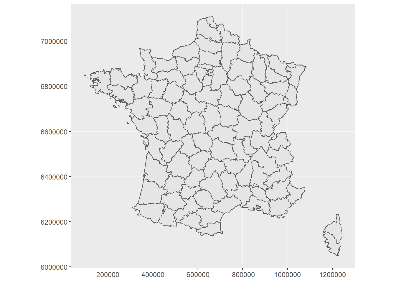
So far, so good. This was the easy part. Now, let’s go back to joining station location and station users’s data.
Joining station files
I am not even going to try to attempt to join files using station names. There is a UIC code, that is, the international railway code, and if it is not working, I am burning the directory and never touching a SNCF file ever again.
In the station_list file, the UIC codes are numeric, let’s put them in character, as in the other file. Also, the station list has stations that are not open for public (only fret trains), we filter them out.
station_list_voyageurs <- mutate(station_list,
                                 code_uic = as.character(code_uic)) %>%
  filter(voyageurs == "O")
Now we go for the join! (hold one’s breath)
station_all <- left_join(station_list_voyageurs,
                         station_freq,
                         by = c("code_uic" = "code_uic"))
Good sign, the number of lines remained the same. Let’s look.
head(station_all) %>% select(code_uic, nom_de_la_gare)## # A tibble: 6 x 2
## code_uic nom_de_la_gare
## <chr> <chr>
## 1 87342139 <NA>
## 2 87342048 <NA>
## 3 87334508 <NA>
## 4 87342105 <NA>
## 5 87342006 <NA>
## 6 87328021 <NA>NA, NA, NA, NA… It’s NA all the way down.
Why?
Well, apparently, the UIC codes differ in the two files.
How naïve of me to have assumed that the SNCF would harmonize the International Railway codes of their stations between their files.
Upon inspection, it seems that there is a “87” in front of all UIC codes in the station_list file. I have no interest in knowing why, I will remove it (dirtily) and hope for the best.
station_list_voyageurs <- mutate(station_list_voyageurs,
                                 CODE_UIC_BETTER_BE_GOOD = str_replace(code_uic,
                                                                       "87",
                                                                       ""))

station_all <- left_join(station_freq,
                         station_list_voyageurs,
                         by = c("code_uic" = "CODE_UIC_BETTER_BE_GOOD"))
So now I have more lines in the file after the left join, which suggests that they were duplicates with the same UIC code.
station_list_voyageurs %>%
  arrange(libelle_gare) %>%
  head()
## # A tibble: 6 x 17
## code_uic libelle_gare fret voyageurs code_ligne rang pk commune
## <chr> <chr> <chr> <chr> <dbl> <dbl> <chr> <chr>
## 1 87313759 Abancourt N O 325000 2 0+000 Abanco~
## 2 87313759 Abancourt N O 321000 1 50+8~ Abanco~
## 3 87313759 Abancourt N O 325000 1 125+~ Abanco~
## 4 87481614 Abbaretz N O 519000 1 469+~ Abbare~
## 5 87317362 Abbeville O O 289000 1 134+~ <NA>
## 6 87317362 Abbeville O O 311000 1 175+~ Abbevi~
## # ... with 9 more variables: departement <chr>, idreseau <dbl>,
## # idgaia <chr>, x_lambert93 <dbl>, y_lambert93 <dbl>, x_wgs84 <dbl>,
## # y_wgs84 <dbl>, coordonnees_geographiques <chr>,
## # CODE_UIC_BETTER_BE_GOOD <chr>Obviously, some stations are represented several times. It’s fine, I just need one of them.
station_list_voyageurs <- station_list_voyageurs %>%
  drop_na(x_lambert93) %>%
  drop_na(y_lambert93) %>%
  filter(!duplicated(libelle_gare))
station_all <- left_join(station_freq,
station_list_voyageurs,
by = c("code_uic" = "CODE_UIC_BETTER_BE_GOOD"))The number of lines remained the same.
station_all %>% head()## # A tibble: 6 x 24
## nom_de_la_gare nb_plate_formes nom_de_la_plate~ code_uic code_postal
## <chr> <dbl> <chr> <chr> <dbl>
## 1 Les Yvris Noi~ 1 Les Yvris Noisy~ 113803 93160
## 2 Les Rosiers-s~ 1 Les Rosiers-sur~ 487876 49350
## 3 Lézignan-Corb~ 1 Lézignan-Corbiè~ 615112 11200
## 4 Les Versannes 1 Les Versannes 595702 24330
## 5 Libourne 1 Libourne 584052 33500
## 6 Les Tines 1 Les Tines 746834 74400
## # ... with 19 more variables: segmentation <chr>,
## # total_voyageurs_2017 <dbl>, total_voyageurs_2016 <dbl>,
## # code_uic.y <chr>, libelle_gare <chr>, fret <chr>, voyageurs <chr>,
## # code_ligne <dbl>, rang <dbl>, pk <chr>, commune <chr>,
## # departement <chr>, idreseau <dbl>, idgaia <chr>, x_lambert93 <dbl>,
## # y_lambert93 <dbl>, x_wgs84 <dbl>, y_wgs84 <dbl>,
## # coordonnees_geographiques <chr>station_all %>% tail()## # A tibble: 6 x 24
## nom_de_la_gare nb_plate_formes nom_de_la_plate~ code_uic code_postal
## <chr> <dbl> <chr> <chr> <dbl>
## 1 Walbourg 1 Walbourg 213405 67360
## 2 Xeuilley 1 Xeuilley 141549 54990
## 3 Wambaix 1 Wambaix 345595 59400
## 4 Zetting 1 Zetting 193649 57115
## 5 Zu Rhein 1 Zu Rhein 472639 68200
## 6 Yvetot 1 Yvetot 413385 76190
## # ... with 19 more variables: segmentation <chr>,
## # total_voyageurs_2017 <dbl>, total_voyageurs_2016 <dbl>,
## # code_uic.y <chr>, libelle_gare <chr>, fret <chr>, voyageurs <chr>,
## # code_ligne <dbl>, rang <dbl>, pk <chr>, commune <chr>,
## # departement <chr>, idreseau <dbl>, idgaia <chr>, x_lambert93 <dbl>,
## # y_lambert93 <dbl>, x_wgs84 <dbl>, y_wgs84 <dbl>,
## # coordonnees_geographiques <chr>Perfect.
We check if there are duplicates in the station names. Yes we have.
station_all %>%
  get_dupes(nom_de_la_gare) %>% view()
The duplicates don’t seem to be mistakes, but stations with different substations (TGV and TER for example). We will thus add the number of passengers per station. And pick one set of coordinates, arbitrarily, the smallest.
station_all <- station_all %>%
  group_by(nom_de_la_gare, departement) %>%
  summarise(total_voyageurs_2017 = sum(total_voyageurs_2017),
            x_lambert93 = min(x_lambert93),
            y_lambert93 = min(y_lambert93))
At the level of France
First, let’s plot all passenger stations.
france +
  geom_point(data = station_list,
             aes(x = x_lambert93,
                 y = y_lambert93),
             size = 0.1,
             colour = "red", alpha = 0.7) +
  labs(title = "French passenger train stations")
## Warning: Removed 890 rows containing missing values (geom_point).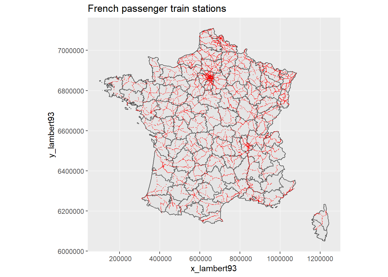
We get a first feel of the distribution of train stations. Mountain areas have lower coverage (Alps in the South east, Pyrennees in the South West, along the Spain border, Corsica.).
france +
  geom_point(data = station_all %>%
               filter(total_voyageurs_2017 >  500000),
             aes(x = x_lambert93,
                 y = y_lambert93),
             size = 0.4,
             colour = "red", alpha = 0.7) +
  labs(title = "French passenger train stations",
       subtitle = "Stations with more than 500 000 passengers in 2017")
## Warning: Removed 7 rows containing missing values (geom_point).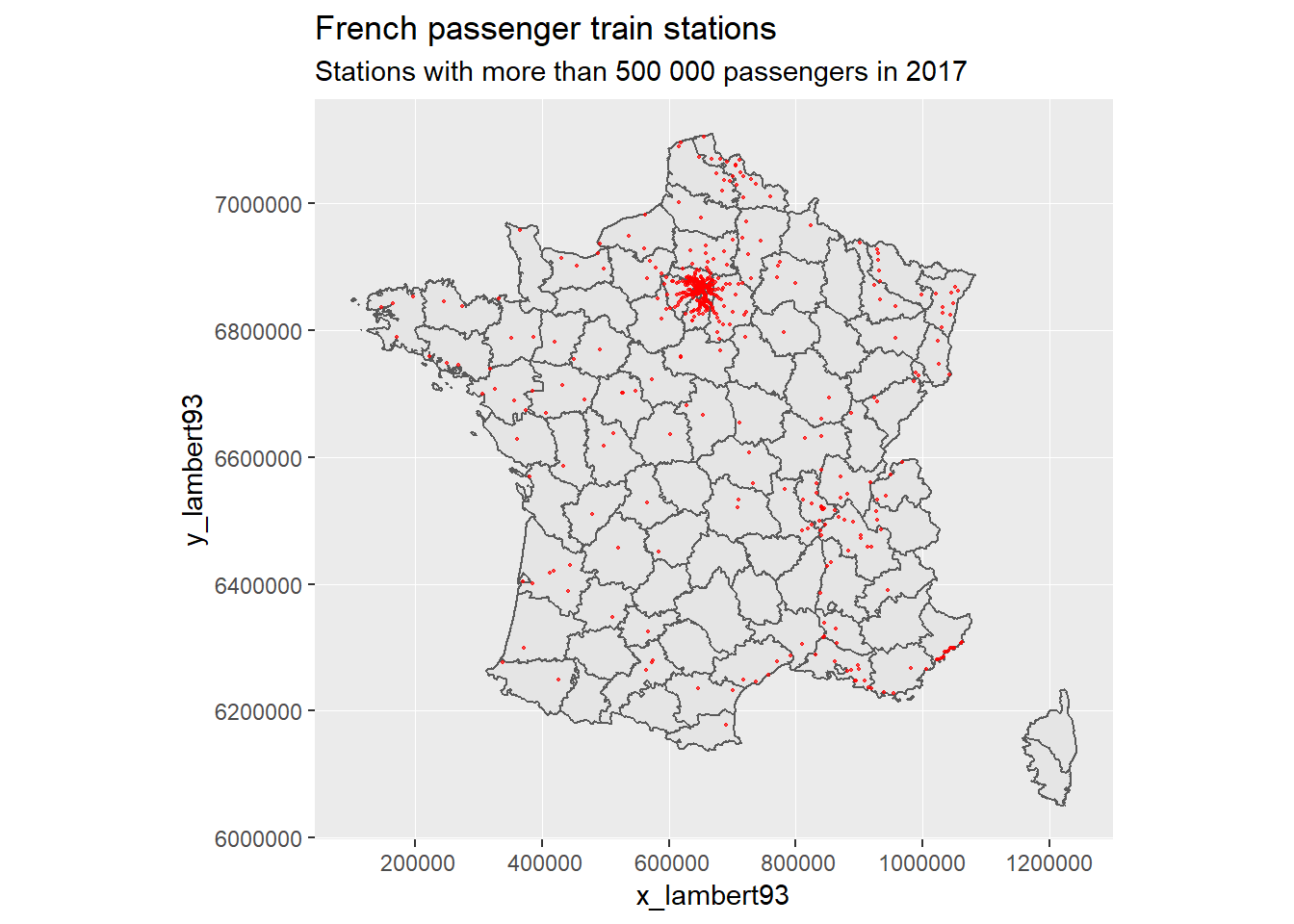
The stations in the Paris region are awfully crowded. The Rhone-Alpes region, as well as along the Mediterranean region have a decent coverage as well. And we can see what French people call “the empty diagonal”, with a much lower number of inhabitant reflected in this dataset.
OK, now we want to add the passenger data on the map. To get a feel of the number of passengers in the largest stations, let’s sort the file.
station_all %>%
  select(nom_de_la_gare, total_voyageurs_2017) %>%
  filter(total_voyageurs_2017 >  10000000) %>%
  arrange(desc(total_voyageurs_2017))
## # A tibble: 48 x 2
## # Groups: nom_de_la_gare [47]
## nom_de_la_gare total_voyageurs_2017
## <chr> <dbl>
## 1 Total 2591307045
## 2 Paris Gare du Nord 211771117
## 3 Paris Saint-Lazare 107875417
## 4 Paris Gare de Lyon 100560512
## 5 Paris Montparnasse 54194496
## 6 Haussmann Saint-Lazare 44647200
## 7 Magenta 41256000
## 8 Juvisy 38195637
## 9 Paris Est 35411032
## 10 Lyon Part Dieu 31884905
## # ... with 38 more rowsThere was a “Total” line somewhere. I am against this kind of practice. Let’s get rid of it.
station_all <- filter(station_all,
                      nom_de_la_gare != "Total")
france +
geom_point(data = station_all %>%
filter(total_voyageurs_2017 > 500000) %>%
arrange(total_voyageurs_2017),
aes(x = x_lambert93,
y = y_lambert93,
colour = log(total_voyageurs_2017),
size = log(total_voyageurs_2017)),
alpha = 0.7) +
labs(title = "French passenger train stations",
subtitle = "Stations with more than 500 000 passengers in 2017",
x = "",
y = "",
caption = "Source: data.sncf.com") +
scale_color_viridis_c(limits = c(14, 19),
breaks = seq(14, 19,
by = 1),
guide = guide_legend(reverse = TRUE),
name = "Log(Nb of passengers)",
option = "magma",) +
scale_size_continuous(limits = c(14, 19),
breaks = seq(14, 19,
by = 1),
guide = guide_legend(reverse = TRUE),
name = "Log(Nb of passengers)") +
theme_ipsum_rc()## Warning: Removed 223 rows containing missing values (geom_point).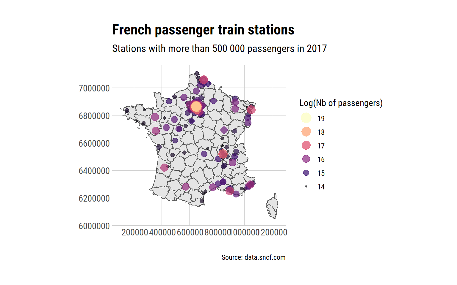
Pretty.
france +
  geom_point(data = station_all %>%
               filter(total_voyageurs_2017 > 5000000) %>%
               arrange(total_voyageurs_2017),
             aes(x = x_lambert93,
                 y = y_lambert93,
                 colour = log(total_voyageurs_2017),
                 size   = log(total_voyageurs_2017)),
             alpha = 0.6) +
  labs(title = "French passenger train stations",
       subtitle = "Stations with more than five millions passengers in 2017",
       x = "",
       y = "",
       caption = "Source: data.sncf.com") +

  scale_color_viridis_c(limits = c(14, 19),
                        breaks = seq(14, 19,
                                     by = 1),
                        option = "magma",
                        guide = guide_legend(reverse = TRUE),
                        name = "Log(Nb of passengers)") +
  scale_size_continuous(limits = c(14, 19),
                        breaks = seq(14, 19,
                                     by = 1),
                        guide = guide_legend(reverse = TRUE),
                        name = "Log(Nb of passengers)") +
  theme_ipsum_rc()
## Warning: Removed 4 rows containing missing values (geom_point).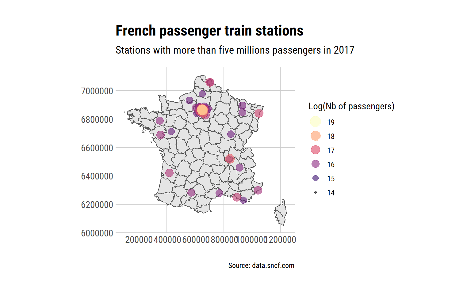
Without the size dependence of points.
france +
  geom_point(data = station_all %>%
               filter(total_voyageurs_2017 > 5000000) %>%
               arrange(total_voyageurs_2017),

             aes(x = x_lambert93,
                 y = y_lambert93,
                 colour = log(total_voyageurs_2017)),

             alpha = 0.5) +

  labs(title = "French passenger train stations",
       subtitle = "Stations with more than five millions passengers in 2017",
       x = "",
       y = "",
       caption = "Source: data.sncf.com") +

scale_color_viridis_c(option = "magma",
                      guide = guide_legend(reverse = TRUE),
                      name = "Log(Nb of passengers)")
## Warning: Removed 3 rows containing missing values (geom_point).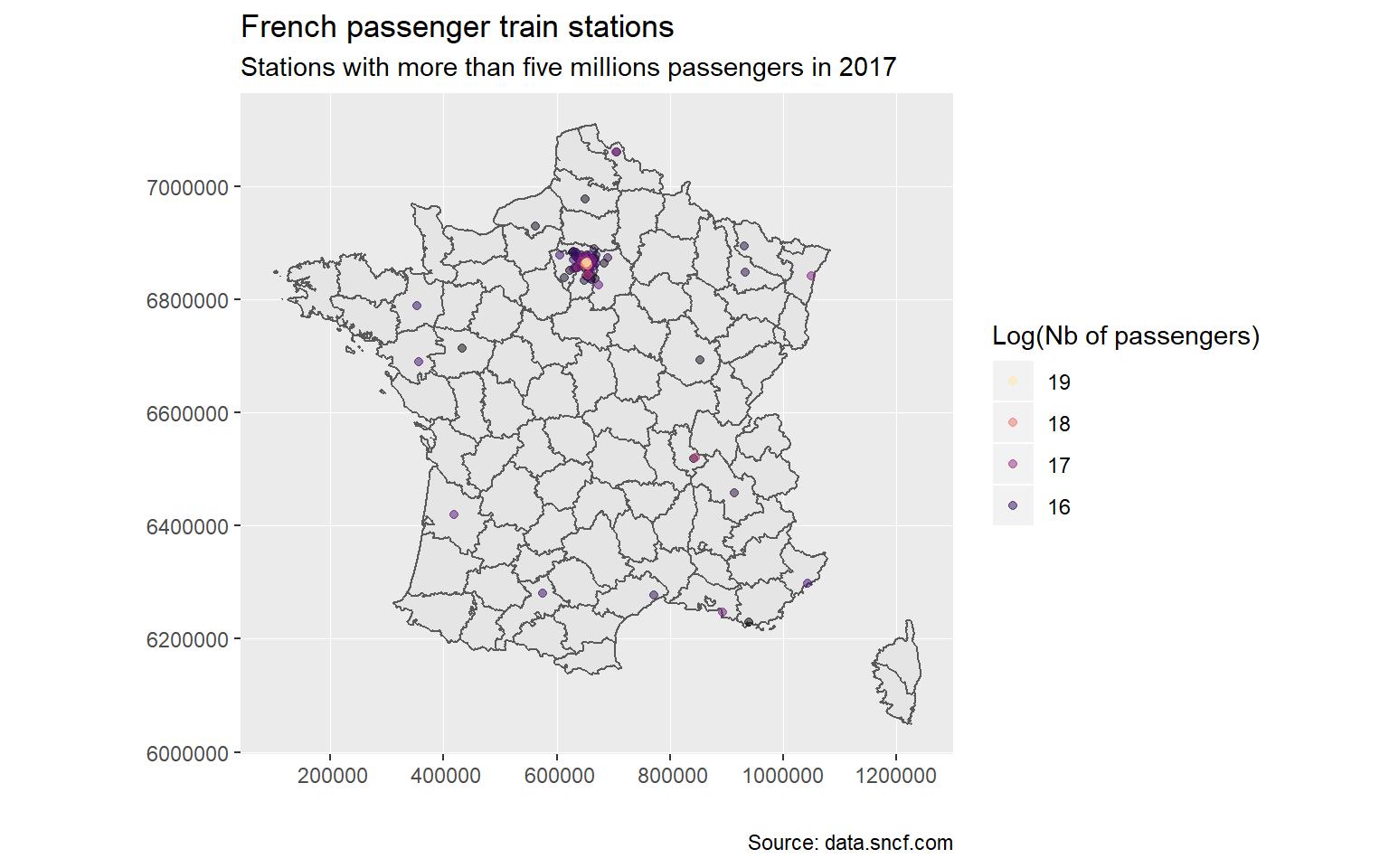
The Paris region has very, very high numbers of passengers per year. For the rest, we see the big towns.
Paris region (Ile-de-France)
ile_de_france <- departements_L93 %>%
  filter(NOM_REG == "ILE-DE-FRANCE")
idf <- ggplot(ile_de_france) +
scale_fill_viridis_d() +
geom_sf() +
coord_sf(crs = 2154, datum = sf::st_crs(2154)) +
guides(fill = FALSE)
idf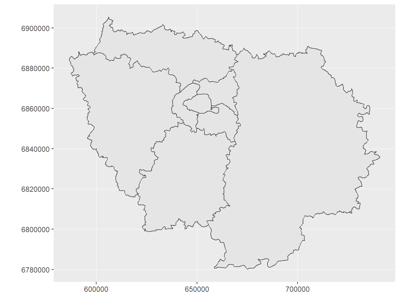
stations_idf <- station_all %>%
  filter(departement %in% c("Seine-St-Denis", "Paris", "Essone", "Yvelines", "Val-d'Oise", "Hauts-de-Seine", "Val-de-Marne", "Seine-et-Marne"))
idf +
geom_point(data = stations_idf %>%
arrange(total_voyageurs_2017),
aes(x = x_lambert93,
y = y_lambert93,
colour = log(total_voyageurs_2017),
size = log(total_voyageurs_2017)),
alpha = 0.7) +
labs(title = "French train stations around Paris",
subtitle = "Ile de France Region (Paris) - 2017",
x = "",
y = "",
caption = "Source: data.sncf.com") +
scale_color_viridis_c(limits = c(10, 18),
breaks = seq(10, 18,
by = 1),
option = "magma",
guide = guide_legend(reverse = TRUE),
name = "Log(Nb of passengers)") +
scale_size_continuous(limits = c(10, 18),
breaks = seq(10, 18,
by = 1),
guide = guide_legend(reverse = TRUE),
name = "Log(Nb of passengers)") +
theme_ipsum_rc()## Warning: Removed 3 rows containing missing values (geom_point).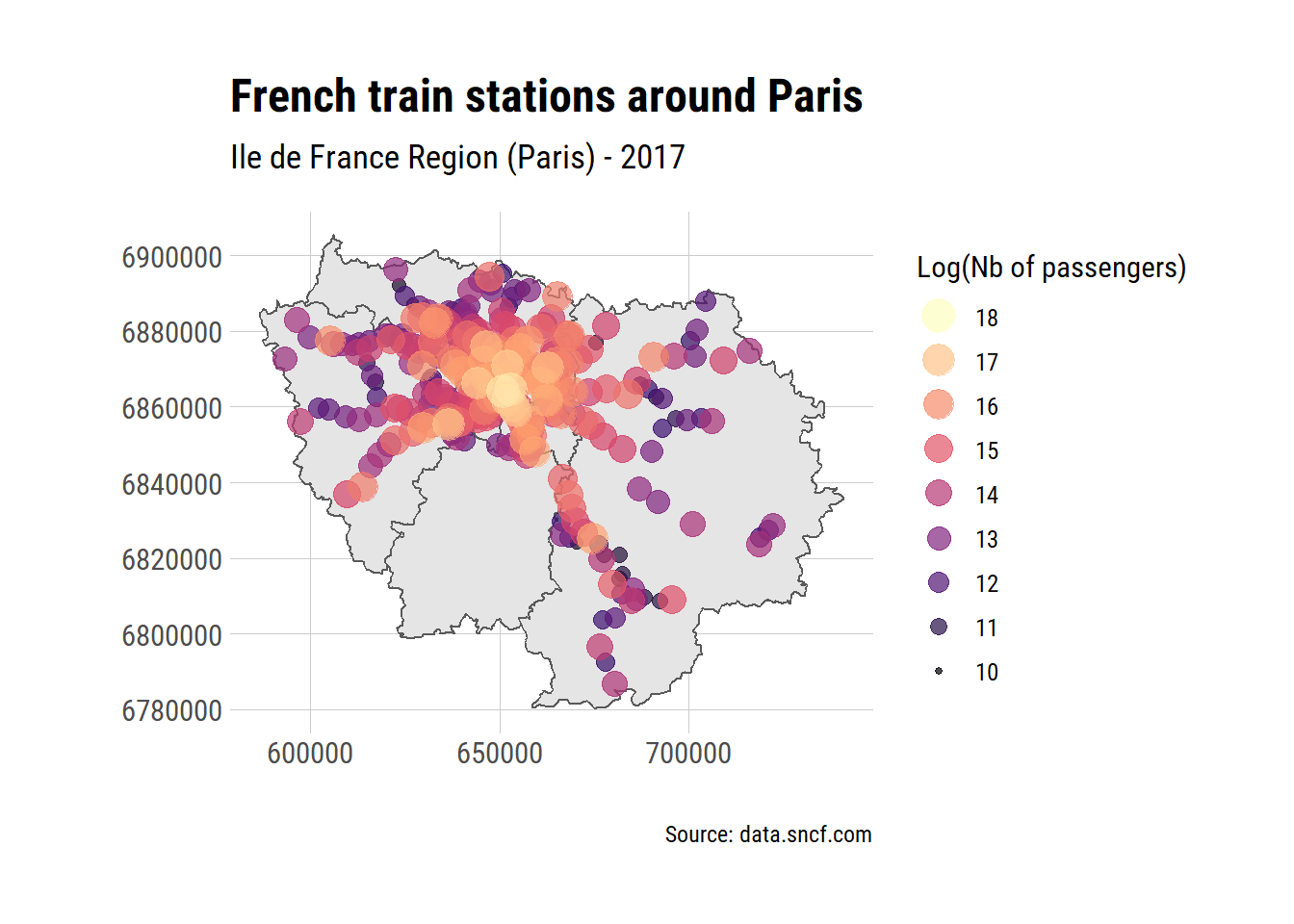
We can see the lines leaving Paris for the surrounding areas. They get less and less passengers the further they go.
And that is all for today.
(I think that UIC stands for Union Inter des Chemins de fer)↩
Like write two or three papers, apply for jobs, enjoy South of France amazing spring and plot network of evolutionary scientists as measured through PhD commitees, you know, the fun things in life↩
That is a reference only French people can understand I am afraid↩
Why are these not in the station reference list, we shall never know↩