Introduction

Some months ago, I donwloaded the summary file of all PhD theses defended in France from 1986 to 2018, as they appear in the national database these.fr. One of the national database, at least¹.

It is a big file, with 369554 lines (at the date I downloaded it), and there are many things to investigate with it. Today I focus on a network analysis, inspired by the great posts of Baptiste Coulmont and Olivier Gimenez, who respectively conducted such an analysis in social sciences and ecology. Being an evolutionnary biologist, I had to do one in evolution.

I modified the code from Olivier Gimenez to apply it to French evolutionary biologists. Or rather, evolutionary biologists that are involved in supervising and evaluating PhDs (a process which also involves non-French scientists).

Getting all the data

Get PhD data

I downloaded and cleaned the whole file from theses.fr using the following commands. Beware, it takes some time.

i <- 1:400
i <- i*1000

URL <- paste0("https://www.theses.fr/?q=&fq=dateSoutenance:[1965-01-01T23:59:59Z%2BTO%2B2018-12-31T23:59:59Z]&checkedfacets=&start=",i, "&sort=none&status=status:soutenue&access=&prevision=&filtrepersonne=&zone1=titreRAs&val1=&op1=AND&zone2=auteurs&val2=&op2=AND&zone3=etabSoutenances&val3=&op3=AND&zone4=dateSoutenance&val4a=&val4b=&type=lng=&checkedfacets=&format=csv")

map(URL, getURL) %>% write.csv(.,"./1_raw_data/SERP_2.csv")

thesis <- read.csv("./1_raw_data/SERP_2.csv",
                   sep = ";", quote = "", skip = 1,
                   stringsAsFactors = F)

# Improve colnames
colnames(thesis) <- c("author", "author_id", "title", 
                      "thesis_advisor1", "thesis_advisor2", "thesis_advisors_id", 
                      "university", "university_id", "discipline", 
                      "status", "date_first_registration", "date_defense", 
                      "language", "thesis_id", 
                      "online", "date_upload", "date_update", "whatever")


# Remove weird column in the end
# Get rid of duplicated header rows & crappy lines
# Put the names of authors or advisors in lower case plus majuscule
# Get date in YMD format
# Get year, month and week onf the day
thesis2 <- thesis %>% 
  select(-whatever) %>% 
  filter(!str_detect(online, "Accessible en ligne")) %>% 
  mutate(author          = str_to_title(author),
         thesis_advisor1 = str_to_title(thesis_advisor1),
         thesis_advisor2 = str_to_title(thesis_advisor2)) %>% 
  filter(title != "",
         status == "soutenue",
         !str_detect("discipline")) %>% 
  mutate(date_first_registration = dmy(date_first_registration),
         date_defense            = dmy(date_defense),
         date_update             = dmy(date_update),
         date_upload             = dmy(date_upload)) %>% 
  mutate(year_defense  = year(date_defense),
         month_defense = month(date_defense, label = TRUE, abbr = FALSE),
         day_defense   = wday(date_defense,  label = TRUE, abbr = FALSE)) %>% 
  mutate(title = str_replace(title, "\"\"", "")) %>% 
  mutate(title = str_replace(title, "\"", "")) %>% 
  
  filter(!str_detect(title, "Fa yan kan zhong guo"))


# Save
write.table(thesis2, 
            "./2_clean_data/thesis.csv",
            quote = FALSE,
            sep = ";",
            dec = ".",
            row.names = FALSE)

Get evolution-related PhD

I want the PhDs from the evolutionary field. It is a bit tricky because the field name (discipline in the dataframe) depends on doctoral schools, and changes every couple of years within doctoral schools.

I first filtered by discipline names that contain variation on the word evolution (“Évolut|Evolut|evolut|évolut|”) using the str_detect() function from the excellent stringr package.

I obtained a couple of fields that have nothing to do with evolutionary biology. For example, “evolution of terrestrial systems”. Fortunately, the list of fields was not so long, so I could check it and manually filter out fields that really did not belong (mostly from geology and earth sciences).

We can see that there are fields which include evolution but are much larger, such as “biological sciences and evolution”, but I don’t think much can be done about it.

Then I noticed that I had very few PhDs from before 2000, so I spent a couple of minutes searching for the PIs in my lab, and got some more fields to add. I am sure that we are missing some people², but I think we got the bulk of evolutionary biology PhDs.

thesis_evolution <- thesis %>% 
  filter(str_detect(discipline, 
                    pattern = "Évolut|Evolut|evolut|évolut|Genetique des populations") |
           discipline %in% c("Physiologie et biologie des organismes et populations", "Biologie des populations et ecologie")) %>% 
  drop_na(date_defense) %>% 
  filter(!str_detect(discipline,
                   pattern = "Terre|planete|lithos|geologie|Geologie|evolutionnaire|Materiaux|materiaux"))

We now have 1180 PhD, from 1986 to 2018.

We can look at the distribution of the year of defense. I don’t know whether the lower number of PhDs in the late nineties are because of a large shift towards a different name for the fields or some real temporary loss of interest in evolutionary biology. I would wagger on the former.

thesis_evolution %>% 
  ggplot(aes(x = date_defense)) +
  geom_histogram() +
  theme_ipsum_rc() +
  labs(title = "Nb of PhD defended in evolution, 1986 - 2018",
       subtitle = "Obviously, some are missing",
       x = "Year",
       y = "Nb of defended PhD",
       caption = "Data: theses.fr")

## `stat_bin()` using `bins = 30`. Pick better value with `binwidth`.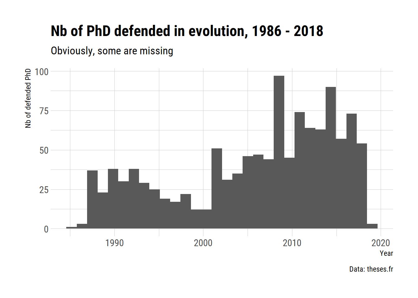

Get advisor ans commitees data

Now that we have the ID of the PhDs related to evolution, we need to get the data about the advisors and the commitees related to these PhDs. To do that, we scrap the webpage of each PhD (using the PhD ID) using the rvest package.

thesis_id <- thesis_evolution$thesis_id # get PhD ids

total_network <- data.frame(jury_members = "",
                            jury_links = "",
                            these      = "",
                            directeurs = "",
                            advisor_id = "")


for (i in 1:length(thesis_id)) {
  
  # get info on current PhD
  data_phd_evolution <- read_html(paste0("http://www.theses.fr/",
                                      thesis_id[i]) ) 
  
  # get name PhD supervisor for 
  directeurs <- bind_cols(
    directeurs = data_phd_evolution  %>%
      html_nodes("div .donnees-ombre p") %>%
      .[[1]] %>%
      html_nodes("a") %>%
      html_text()
    ,
    advisor_id = data_phd_evolution  %>%
      html_nodes("div .donnees-ombre p") %>%
      .[[1]] %>%
      html_nodes("a") %>%
      html_attr(name="href")
  ) %>% mutate(these = thesis_id[i])
  
 
  # get names of people in commitees
  jury <- bind_cols( 
    jury_members = data_phd_evolution %>%
      html_nodes("div .donnees p a") %>%
      html_text()
    ,
    jury_links = data_phd_evolution %>%
      html_nodes("div .donnees p a") %>%
      html_attr(name="href")
  ) %>% mutate(  these = thesis_id[i] )
  
  # put all together
  network <- jury %>% left_join(directeurs,by="these") 
  total_network <- bind_rows(total_network, network)
}

# Because the process is a bit long, we save the file
save(thesis_evolution,
     total_network,
     file = "2019-03-05-network_total.RData")

Building the network

Baptiste Coulmont weighted the different types of links between scientists depending on their role in the PhD process.

If two scientists co-supervise a PhD, the link has a weight of 3, because we assume that co-supervising a PhD student creates or is the consequence of a strong link.
If one of them is a supervisor and the other is in the PhD commitee, the link has a weight 2, indicating a moderate link.
If both researchers are in the same committee, the weight is 1.

The weight of these links can be added (a lot of people are involved both in co-supervisions and commitees).

# Link supervisor - supervisor
advisor_advisor <- total_network %>% 
  select(these, directeurs) %>% 
   mutate(directeurs = str_trim(directeurs)) %>% 
  unique() %>% 
  group_by(these) %>% 
  mutate(N = n()) %>%
  
  filter(N == 2) %>% # keep co-supervision w/ 2 supervisors 
  mutate(rang  = rank(directeurs)) %>% 
  spread(key   = rang, 
         value = directeurs) %>% 
  
  ungroup() %>% 
  select(name_1 = `1`, name_2 = `2`) %>% 
  mutate(poids = 3)


# Link advisor - jury
advisor_jury <- total_network %>% 
  
  select(name_1 = jury_members,
         name_2 = directeurs) %>% 
  
      mutate(name_1 = str_trim(name_1),
           name_2 = str_trim(name_2)) %>% 
  
  filter( name_1 != "") %>%
  mutate(poids = 2) %>%
  group_by(name_1, name_2) %>% 
  # Sum weight over links
  summarize(poids = sum(poids))

# Jury - jury links
jury_jury <- total_network %>% 
  select(jury_members,these) %>% 
  unique() %>% 
  filter(jury_members != "")

Here are what the files look like:

head(advisor_advisor)

## # A tibble: 6 x 3
##   name_1                     name_2           poids
##   <chr>                      <chr>            <dbl>
## 1 Domitien Debouzie          Frédéric Menu        3
## 2 Brigitte Crouau-Roy        Evelyne Heyer        3
## 3 François Mallet            Laurent Duret        3
## 4 Louis Deharveng            Thierry Deuve        3
## 5 Antoine Kremer             Sophie Gerber        3
## 6 Marie-Catherine Boisselier Philippe Bouchet     3

head(advisor_jury)

## # A tibble: 6 x 3
## # Groups:   name_1 [2]
##   name_1                 name_2               poids
##   <chr>                  <chr>                <dbl>
## 1 Abdelaziz Heddi        Fabrice Vavre            2
## 2 Abdelaziz Heddi        Frédéric Fleury          2
## 3 Abdelaziz Heddi        Mylène Weill             2
## 4 Abdelaziz Heddi        Olivier Duron            2
## 5 Abdelhamid El Mousadik Bouchaïb Khadari         2
## 6 Abdelhamid El Mousadik Cherkaoui El Modafar     2

head(jury_jury)

##        jury_members        these
## 1 Michel Boulétreau 1988LYO10171
## 2 Jean-Marc Deragon 2010PERP1263
## 3     Andrew Leitch 2010PERP1263
## 4  Alain Ghesquière 2010PERP1263
## 5      Jérôme Salse 2010PERP1263
## 6 Sébastien Aubourg 2010PERP1263

Make graph

Now we use the graph_from_data_frame() from the igraph package to create the graph.

# Make non-directed graph for jur_jury
g_j <- graph_from_data_frame(jury_jury,
                              directed = F)

 
# Create the vertex sequence
igraph::V(g_j)$type <- V(g_j)$name %in% jury_jury$jury_members

g_j_1 <- bipartite_projection(g_j, which = "true")


jurys <- as_long_data_frame(g_j_1) %>%
  select(name_1 = `ver[el[, 1], ]`, 
         name_2 = `ver2[el[, 2], ]`, 
         poids  = weight)

reseau_petit <- bind_rows(advisor_advisor,
                          advisor_jury,
                          jurys) %>%
  group_by(name_1, name_2) %>% 
  summarize(poids = sum(poids)) # data.frame from which the network will be created

## Warning in bind_rows_(x, .id): binding character and factor vector,
## coercing into character vector

## Warning in bind_rows_(x, .id): binding character and factor vector,
## coercing into character vector

Plot the network

We correlate the size of the point to betweenness of nodes. The width of the edges correlates with the summed weight of the link between the two scientists (the strenght of their connection).

We determine communities trough a cluster_walktrap algorithm. The cluster_walktrap() function, from the igraph package tries to find densely connected subgraphs (communities) via random walks. The idea is that short random walks tend to stay in the same community. To be honest, it’s mainly to add colour to the graph.

g <- graph_from_data_frame(reseau_petit, 
                           directed = F) 

# Simplfy the graph by removing the identic loops (summing their links)
g <- simplify(g, edge.attr.comb = sum)

V(g)$degres <- degree(g)

# Get surname only
V(g)$label  <- gsub("^\\S+\\s+(.+)$","\\1",V(g)$name)


# determine communities
# step = the length of the random walk to perform
V(g)$communaute <- as.character(cluster_walktrap(g,
                                                 steps = 10)$membership)  # 15 originellement

V(g)$closeness <- (5*closeness(g))^10

## Warning in closeness(g): At centrality.c:2784 :closeness centrality is not
## well-defined for disconnected graphs

# network metric betweeness
V(g)$btwns       <- betweenness(g) 
V(g)$eigen_centr <- eigen_centrality(g)$vector


# delete edges with weight < 4
g <- delete_edges(g, which(E(g)$poids < 4)) # 5 initiallement


# to which community you belong
V(g)$cluster_number <- clusters(g)$membership 

g <- induced_subgraph(g,
                      V(g)$cluster_number == which( max(clusters(g)$csize) == clusters(g)$csize) )

# width of edge proportional to weight
E(g)$weight <- 1/E(g)$poids 


# do not display all names
V(g)$label <- ifelse(V(g)$degres < 9, 
                     "", 
                     V(g)$label)  # 20 initialement

graphe_1 <- ggraph(g,
                   layout = "igraph",
                   algorithm = "fr") + 
  
  geom_edge_link(aes(width = 0.1*poids), alpha = 0.1, 
                 end_cap   = circle(5, 'mm'), 
                 start_cap = circle(5, 'mm')) +
  
  geom_node_point(aes(size = eigen_centr),
                  color = "white", alpha = 1) +
  
  geom_node_point(aes(color = communaute,
                      size = eigen_centr), 
                  alpha = 0.5) +
  
  scale_size_area(max_size = 20) +
  
  geom_node_text(aes(label = label),
                 size = 2.5, 
                 repel = T,
                 box.padding = 0.15)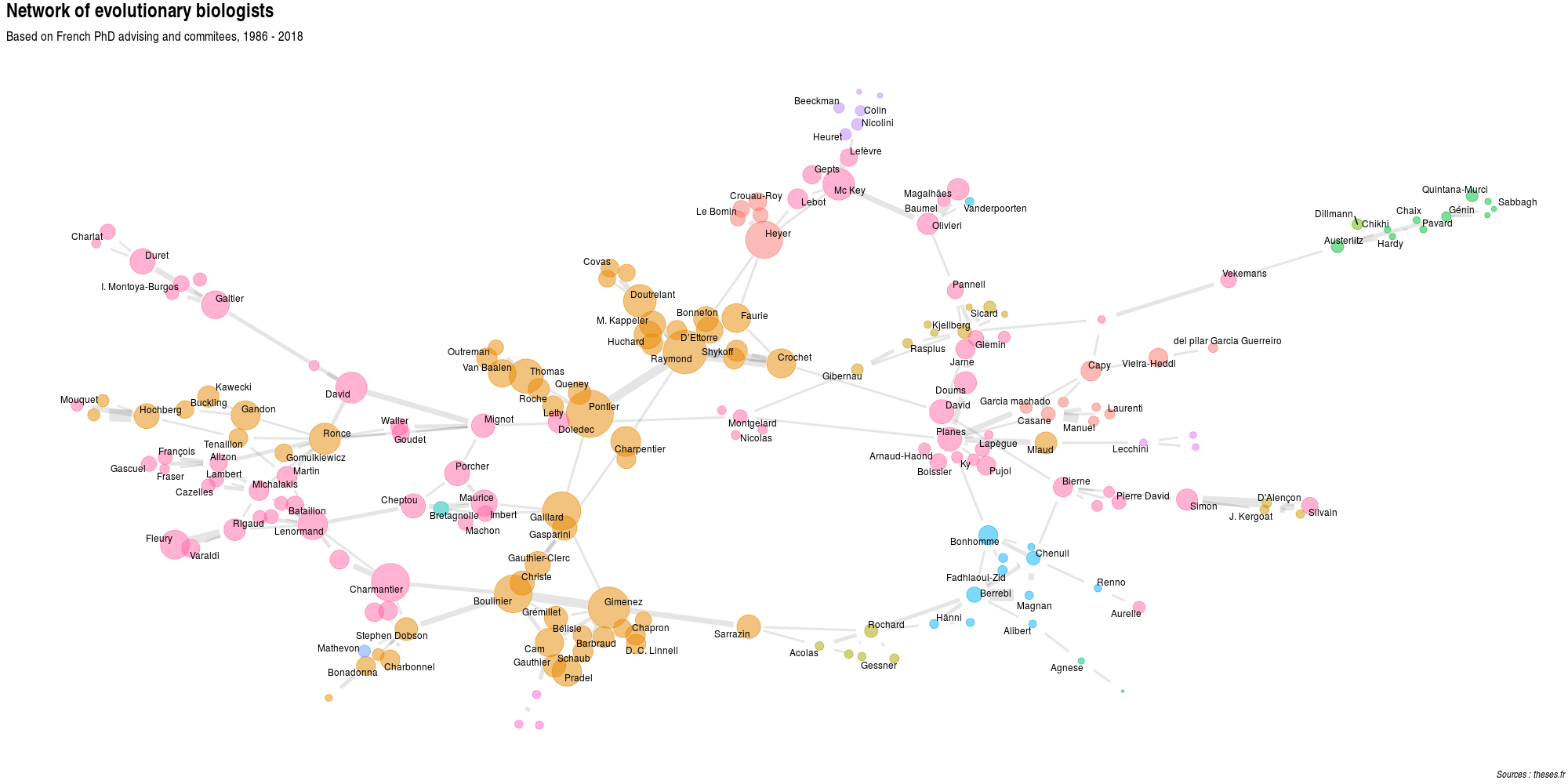

The first thing that I noticed is internal: it is a particularly good feeling when you know the people that are on a figure.

I can recognize groups of people whom I know work and publish together, which is quite reassuring.

At first, I was surprised that people from a same lab were scattered all over the place. However, since PhD commitees must have some proportion of non-local people, there must be connections between people from different labs.

I hope that this also mean something positive about the scientific ties accross labs and France in general.

Plot the network 2015 to 2018

Because the dataset is large, it is difficult to plot more names. So let’s see what the network looks like in the past three years.

I turned the script in functions to perform the same scrapping as above and save some space. See LINK for the source file.

thesis_evolution_2015_2018 <- thesis_evolution %>% 
  filter(year_defense > 2014)

scrapped_2015_2018 <- scrap_phd_webpages(thesis_evolution_2015_2018)

graphe_2 <- make_network_full(scrapped_2015_2018,
                              my_waltrap = 10,
                              my_edge    = 3,
                              my_degree  = 2,
                              my_title   = "Network of evolutionary biologists",
                              my_subtitle = "Based on French PhD advising and commitees, 2015 - 2018")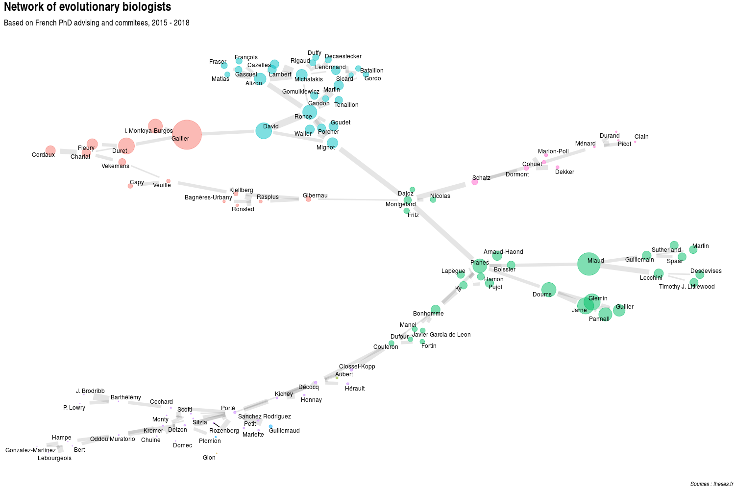

Plot the network in Montpellier

Since I did my PhD in Montpellier, I was very curious to see how the local network is structured.

thesis_evolution_Montpellier <- filter(thesis_evolution,
                             str_detect(university,
                                        pattern = "Montpellier"))

scrapped_Montpellier <- scrap_phd_webpages(thesis_evolution_Montpellier)

graphe_3 <- make_network_full(scrapped_Montpellier,
                              my_waltrap = 10,
                              my_edge    = 4,
                              my_degree  = 5,
                              my_title   = "Network of evolutionary biologists",
                              my_subtitle = "Based on French PhD advising and committes, Montpellier")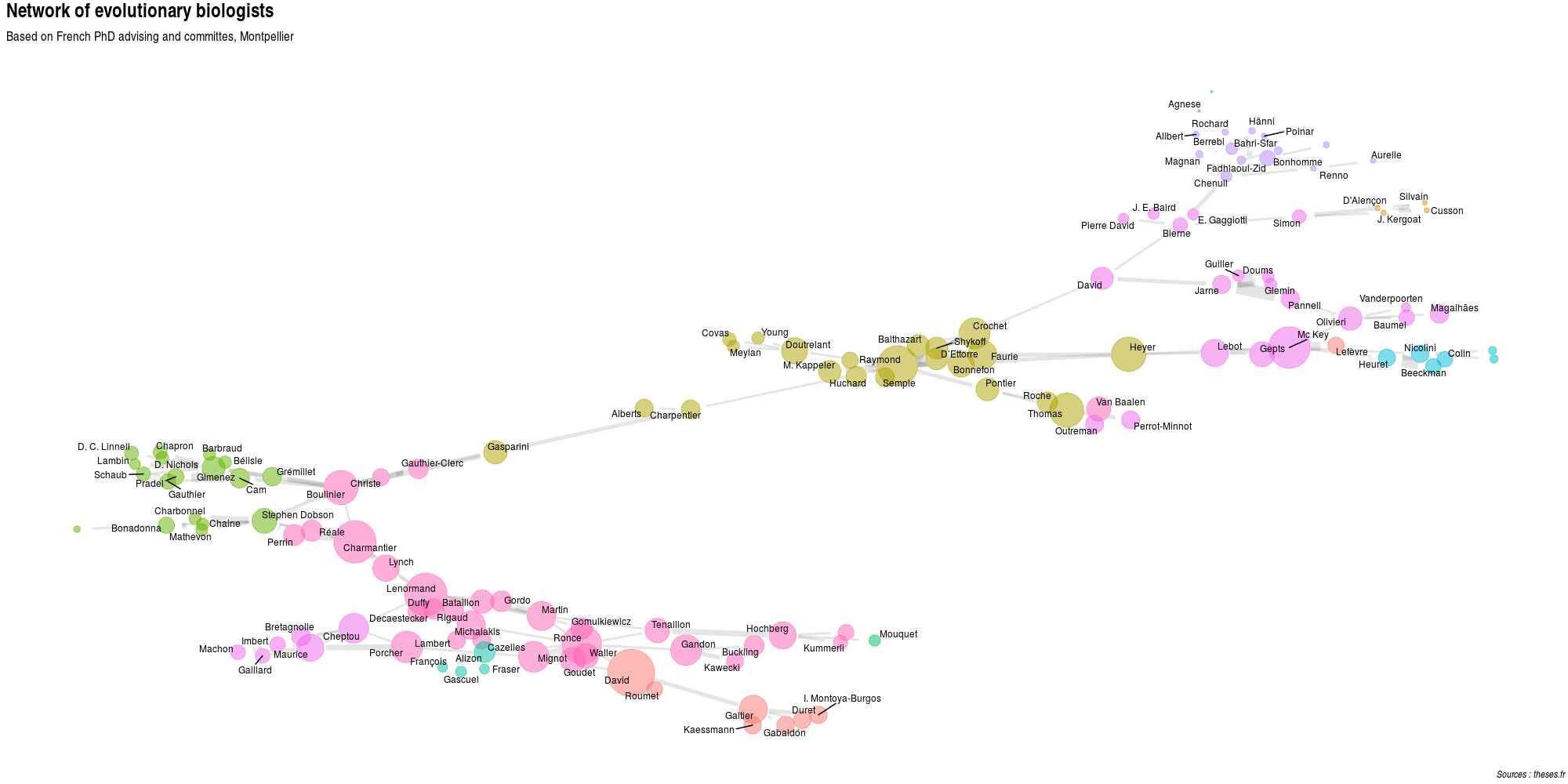

{{ range $i := (slice "categories" "tags") }} {{ with ($.Param $i) }} {{ $i | title }}: {{ range $k := . }} {{$k}} {{ end }} {{ end }} {{ end }}

I heard that the file has a slighly different number of lines than the file downloaded from HAL, another national archive, but I cannot find the discussion again↩
I know of at least one, but the field is “biology”, and really, it’s too wide!↩

Exploration of French Academic Network in Evolution