Today I will use the tools of the tidyverse to explore a file with the data on PhD defended in France from 1986 to 2018.
I downoalded the fille from the national database these.fr sometimes in December 2018, and then sort of forgot about it. Today, I will do a rough exploration of the number of PhD over time, and on when the PhDs are defended within year.
I thought that it was quite fun that a #Tidytuesday was about US PhDs, when I have wanted to have a look at French PhDs for two months. The discipline field is much less tidy, though, so I will not explore it in this post, and focus on dates.
Data
I downloaded all thesis defended in France and recorded on the theses.fr datatabase on the 14 December 2018. This datafile does not take into account thesis that were never defended, or were still under completion at this date.
The code for the downoading and cleaning can be found in the previous post.
load("2019-03-17-thesis.RData")It is a big file, with 369554 lines (at the date I downloaded it).
A first exploration of the author column using the Viewer pane indicates that they are PhDs with several authors, separated by a comma.
thesis2 %>%
  select(author, author_id, year_defense, discipline) %>%
  filter(str_detect(author, ",")) %>%
  head(10)
## author author_id
## 1 Aurelie, Laure Chabeaud 132126974
## 2 Isabelle Lo Pinto,Mathieu J.c Wong So ,
## 3 Guy Chaudeurge,Annette Chaudeurge 124872247,124872549
## 4 Francois Drouillard,Lionel Druon ,
## 5 Francis Daliphard,Yves Lognone 125125402,125125593
## 6 Jean-Francois Aly,Chantal Marie 126228795,12622885X
## 7 Michele Monjauze,Marie-Madeleine Jacquet 03115316X,032985126
## 8 Evelyne, De Montaudouin 149317492
## 9 Cecile, Elsa Dantzer 071348050
## 10 Veronique Larraillet,Francoise Maszkalo ,
## year_defense
## 1 2008
## 2 1989
## 3 1990
## 4 1990
## 5 1991
## 6 1991
## 7 1987
## 8 2010
## 9 2002
## 10 1990
## discipline
## 1 Genie des procedes
## 2 Medecine generale
## 3 Medecine
## 4 Medecine generale
## 5 Medecine
## 6 Medecine
## 7 Psychologie
## 8 Histoire de l'art
## 9 Sciences biologiques et medicales. Epidemiologie et intervention en sante publique
## 10 Medecine generaleIn the 1467 rows, there is a mix of PhDs with two authors1, and PhDs whose authors filled all their secondary names, with colons. I don’t think I can separate the two cases. Since I am not following each author individualy, it does not matter.
Then, we fix the advisor columns. Right now, the advisor 1 is XY and the advisor 2 is YX. When there are two (or more) advisors, their names are in the same column, separated by a comma. I also suppress the few PhDs that were before 1986, and in 2018, because I don’t have the full 2018 year.
thesis_clean <- thesis2 %>%
  filter(year_defense > 1986,
         year_defense < 2018) %>%
  filter(!duplicated(thesis_id)) %>%
  select(-thesis_advisor2) %>%
  mutate(advisors = str_split(thesis_advisor1, ","))
Number of PhDs defended in France
The number of thesis defended in France has decreased around the 2000, but rose again to similar level as before in the past decade.
thesis_clean %>%
  ggplot(aes(x = year_defense)) +
  geom_histogram(binwidth = 1,
                 fill = bar_col,
                 colour = title_colour) +
  labs(title = "Number of PhD defended in France since 1986",
       subtitle = "",
       caption = "Source: theses.fr",
       x = "Year of PhD defense",
       y = "Number of thesis") +
  my_theme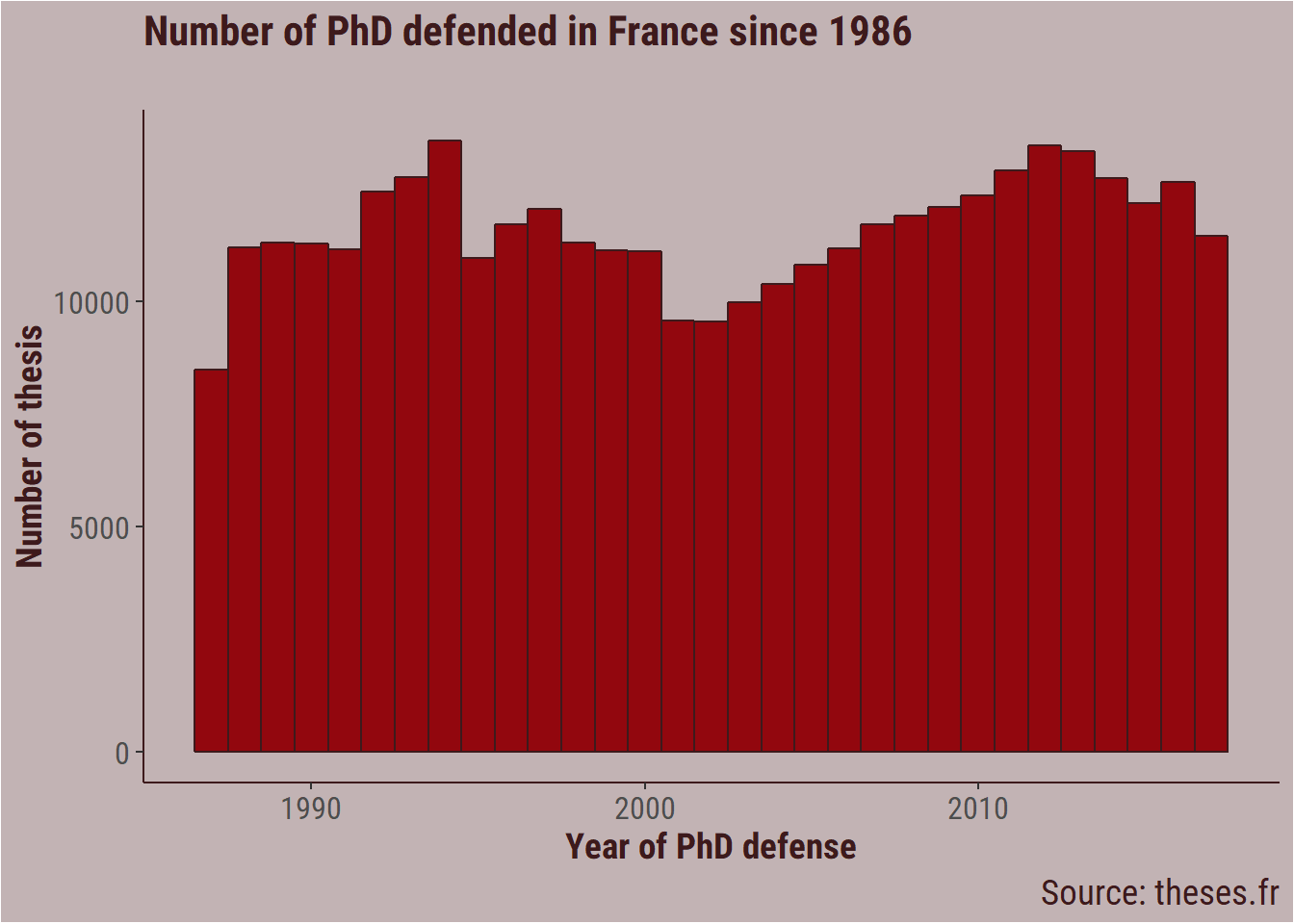
Another way to look at it is with a little animation, using the gganimate package.
p <- thesis_clean %>%
  filter(year_defense < 2018,
         year_defense > 1989) %>%
  group_by(year_defense) %>%
  count() %>%
  ggplot(aes(x = year_defense,
             y = n,
             group = 1)) +
  geom_line(size = 3,
            colour = bar_col) +
  # geom_point(size = 3,
  #            colour = bar_col) +

  labs(title = "Number of PhD defended in France per year",
       subtitle = "",
       caption = "Source: theses.fr",
       x = "Year of defense",
       y = "Number of defended PhDs") +
  ylim(1, 14000) +
  my_theme +

  transition_reveal(year_defense) +
  ease_aes("linear")

animate(p,
        nframes = 100,
        fps = 10)
Number of supervisors
Most PhDs have one or two supervisors. A couple have more.
thesis_clean %>%
  mutate(n_authors = lengths(advisors)) %>%
  count(n_authors) %>%
  mutate(proportion = 100 * n / sum(n))
## # A tibble: 7 x 3
## n_authors n proportion
## <int> <int> <dbl>
## 1 1 295827 82.5
## 2 2 58039 16.2
## 3 3 4496 1.25
## 4 4 388 0.108
## 5 5 22 0.00613
## 6 6 2 0.000557
## 7 7 2 0.000557People with more than one PhDs
There are about 2400 persons with two PhDs (based on author ID). This seems reasonable. Whether the people with four to six PhD represent a mistake in author ID attribution, real PhDs, or crackpots who managed to get a varnish of science is hard to tell.
thesis_clean %>%
  # Remove authors with no ID
  drop_na(author_id) %>%
  filter(author_id != ",",
         !author_id == "") %>%

  count(author_id, sort = TRUE) %>%
  filter(n > 1) %>%

  ggplot(aes(x = n)) +
  geom_histogram(binwidth = 1,
                 fill = bar_col,
                 colour = title_colour) +
  coord_flip() +
  labs(title = "People with more than one PhD",
       subtitle = "Some people hold more than three PhDs... O_O",
       x = "Number of PhDs",
       y = "Number of people",
       caption = "Source: theses.fr") +
  scale_y_continuous(breaks = seq(0, 3000, 200)) +
  my_theme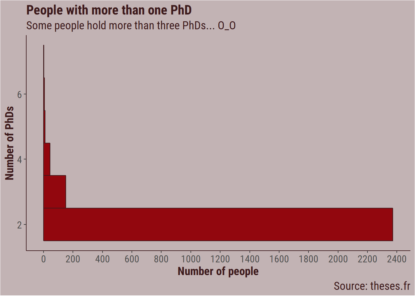
Number of thesis per supervisor
While most people supervised or helped supervise a dozen of PhDs, a decent number of people supervised more than 20 PhDs, which I think is a lot. In France, this is likely to depend on the field. In hard sciences doctoral schools the number of PhD that a PI can supervise at any given time can be limited. I believe that it is a different culture in the humanities.
thesis_clean %>%
  drop_na(thesis_advisors_id) %>%
  filter(!thesis_advisors_id == ",") %>%
  separate_rows(thesis_advisors_id, sep = ",") %>%
  drop_na(thesis_advisors_id) %>%

  group_by(thesis_advisors_id) %>%
  count(thesis_advisors_id, sort = TRUE) %>%
  filter(n < 500) %>%

  ggplot(aes(x = n)) +
  geom_histogram(binwidth = 0.1,
                 fill = bar_col,
                 colour = title_colour) +
  coord_flip() +
   scale_x_continuous(trans = "log10") +
     scale_y_continuous(trans = "log10") +
  labs(title = "Number of PhD supervised by advisor",
       subtitle = "Log10 scale",
       x = "Number of PhDs per (co-)advisor",
       y = "Number of advisors",
       caption = "Source: theses.fr") +
  my_theme
## Warning: Transformation introduced infinite values in continuous y-axis## Warning: Removed 3 rows containing missing values (geom_bar).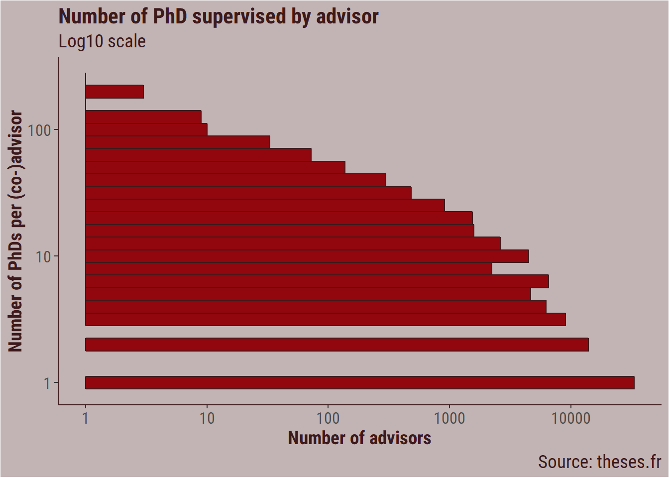
When are PhD defended?
Let’s focus on PhD defended since 2010, and try to use heatmaps to see the patterns across months. Yes, I like heatmaps a bit too much.
Which are the busiest months to defend?
thesis_clean %>%
  filter(year_defense >= 2010) %>%
  mutate(day_defense2 = day(date_defense)) %>%
  group_by(year_defense,
           month_defense,
           day_defense2) %>%
  count() %>%

  ggplot(aes(x = month_defense,
             y = day_defense2,
             fill = n)) +
  facet_wrap(~year_defense, ncol = 8) +
  geom_tile() +

  labs(title = "Distribution of PhD defense over time",
       subtitle = "",
       x = "Month of defense",
       y = "Day of the month") +

  scale_fill_gradient(high = bar_col,
                      low = title_colour) +
   my_theme +
  theme(axis.text.x = element_text(angle = 90,
                                   hjust = 1,
                                  vjust = 0.3))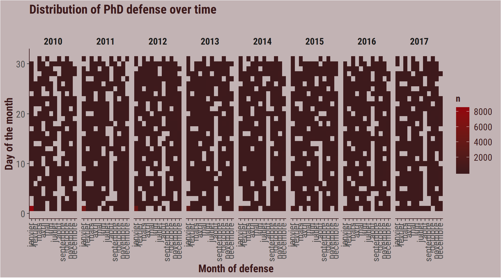
There is a weird pattern, where a lot of PhDs are defended on the first of January in the early year. I suspect tat this represents PhD for which the date of defense was missing, so it got assigned to 01/01.
If we ignore first of January (since it is a holiday in France, it is unlikely that a lot of PhD are really defended on that day, and that it would biais the rest of the dataset).
thesis_clean %>%
  filter(year_defense >= 2010) %>%
  mutate(day_defense2 = day(date_defense)) %>%
  filter(day_defense2 > 1) %>%
  group_by(year_defense,
           month_defense,
           day_defense2) %>%
  count() %>%
  ggplot(aes(x = month_defense,
             y = day_defense2,
             fill = n)) +
  facet_wrap(~year_defense, ncol = 8) +
  geom_tile() +

  labs(title = "Distribution of PhD defense over time",
       subtitle = "",
       x = "Day of the week",
       y = "Defense month") +
  scale_fill_gradient(high = bar_col,
                      low = title_colour) +
  my_theme +
  theme(axis.text.x = element_text(angle = 90,
                                   hjust = 1,
                                   vjust = 0.3))
Now, we begin to see paterns:
- The empty line during the two first weeks of August, when people are on holidays, and most university administration are closed.
- The high numbers in December. This makes sense, because a lot of the PhD begin in september-december. The funding is for three years, and if you begin in September, you have to defend before December three years later. So November and December are busy months for jurys.
Another way to look at it iw with a simple line graph2.
thesis_clean %>%
  filter(year_defense >= 2015,
         year_defense < 2018) %>%
    mutate(year_month = format(as.Date(date_defense),
                              "%Y-%m")) %>%
  group_by(year_defense, month_defense, year_month) %>%
  count() %>%
  ggplot(aes(x = month_defense,
             y = n,
             group = year_defense)) +
  geom_line(colour = bar_col,
            size = 2,
            alpha = 0.7) +
  annotate("text",
           x = "août",
                y = 2000,
                label = "Summer holidays",
                size = 5,
                colour = title_colour) +
  annotate("segment",
           x = "août",
           xend = "août",
           y = 1800,
           yend = 800,
           colour = title_colour,
           size = 1,
           arrow = arrow()) +

  labs(title = "Typical year calendar for PhD defenses (2015-2017)",
       subtitle = "Most PhDs begin in autumn, and they have until December three\nyears later to defend, hence the end-of-year peak",
       x = "Month of defense",
       y = "Number of PhDs",
       caption = "One line = one year\nSource: theses.fr") +
  my_theme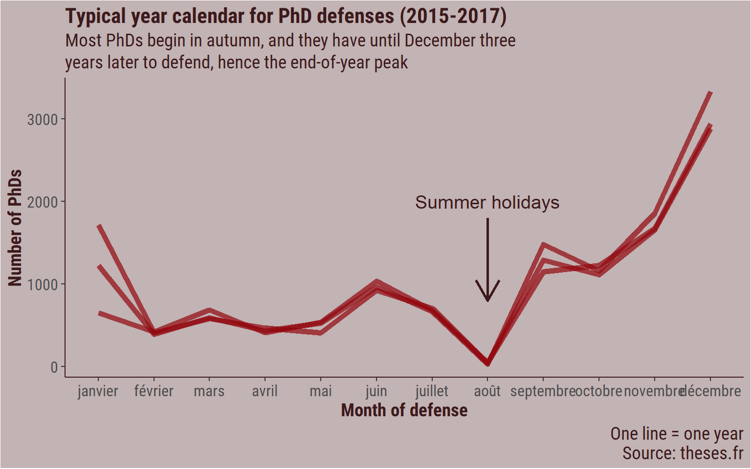
Which days of the week?
thesis_clean %>%
  filter(year_defense >= 2010) %>%
  mutate(day_defense2 = day(date_defense)) %>%
  filter(day_defense2 > 1) %>%
  group_by(year_defense,
           month_defense,
           day_defense) %>%
  count() %>%
  ggplot(aes(x = day_defense,
             y = month_defense,
             fill = n)) +
  facet_wrap(~year_defense, ncol = 8) +
  geom_tile() +

  labs(title = "Distribution of PhD defense over weekdays and months",
       subtitle = "",
       x = "Day of the week",
       y = "Defense month") +

    scale_fill_gradient(high = bar_col,
                      low = title_colour) +
 my_theme +
  theme(axis.text.x = element_text(angle = 90,
                                   hjust = 1,
                                   vjust = 0.3))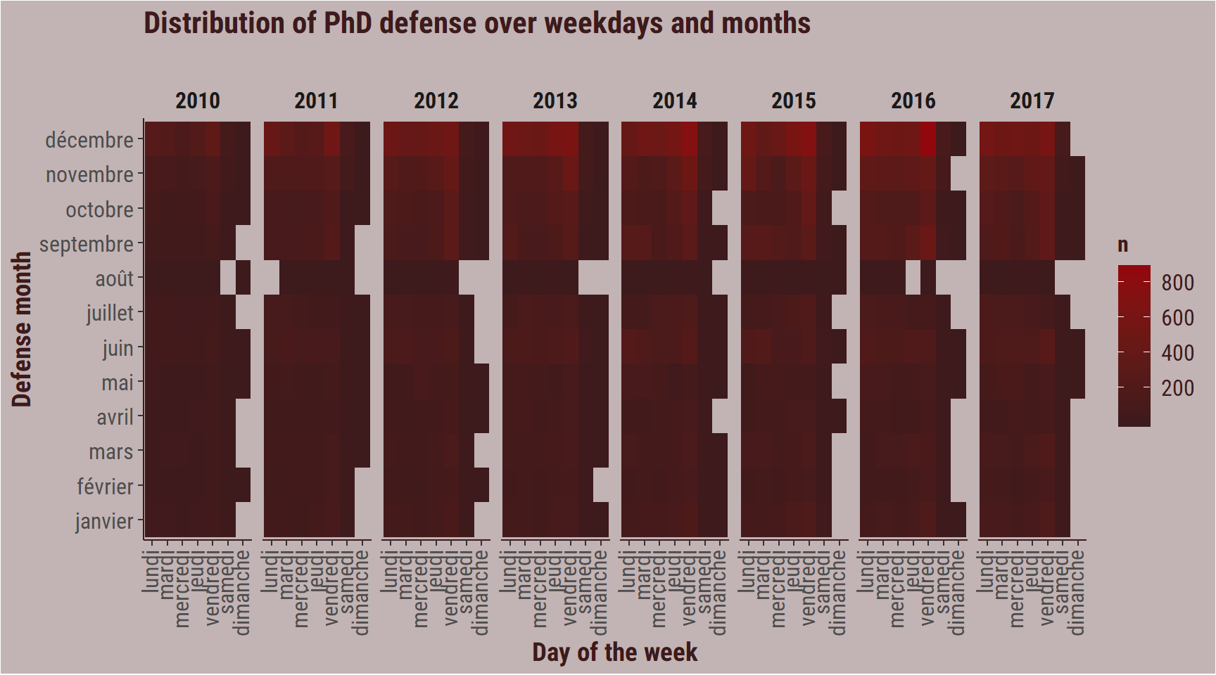
We see the end-of year patterns, but the most interesting observation in my opinion is that there are PhDs defended during the week ends. That is weird.
Ecology and evolution
Since I come from evolutionary ecology, I wanted to have a look at how these fields compare to the pooled data.
Get the data
thesis_evology <- thesis_clean %>%
  filter(str_detect(discipline,
                    pattern = "Évolut|Evolut|evolut|évolut|Genetique des populations|Ecolog|ecolog|écolog|Écolog") |
           discipline %in% c("Physiologie et biologie des organismes et populations", "Biologie des populations et ecologie"))  %>%
  drop_na(date_defense) %>%
  filter(!str_detect(discipline,
                   pattern = "Terre|planete|lithos|geologie|Geologie|evolutionnaire|Materiaux|materiaux|gyneco|Gyneco"))
Defense over time
thesis_evology %>%
  filter(year_defense >= 1990) %>%
  group_by(year_defense) %>%
  ggplot(aes(x = year_defense)) +
  geom_histogram(binwidth = 1,
                 fill   = bar_col,
                 colour = title_colour) +
  labs(title = "Number of PhD defended in ecology and evolution in France",
       subtitle = "From 1990 to 2017",
       x = "Year of PhD defense",
       y = "Number of PhD",
       caption = "Source: theses.fr") +
  my_theme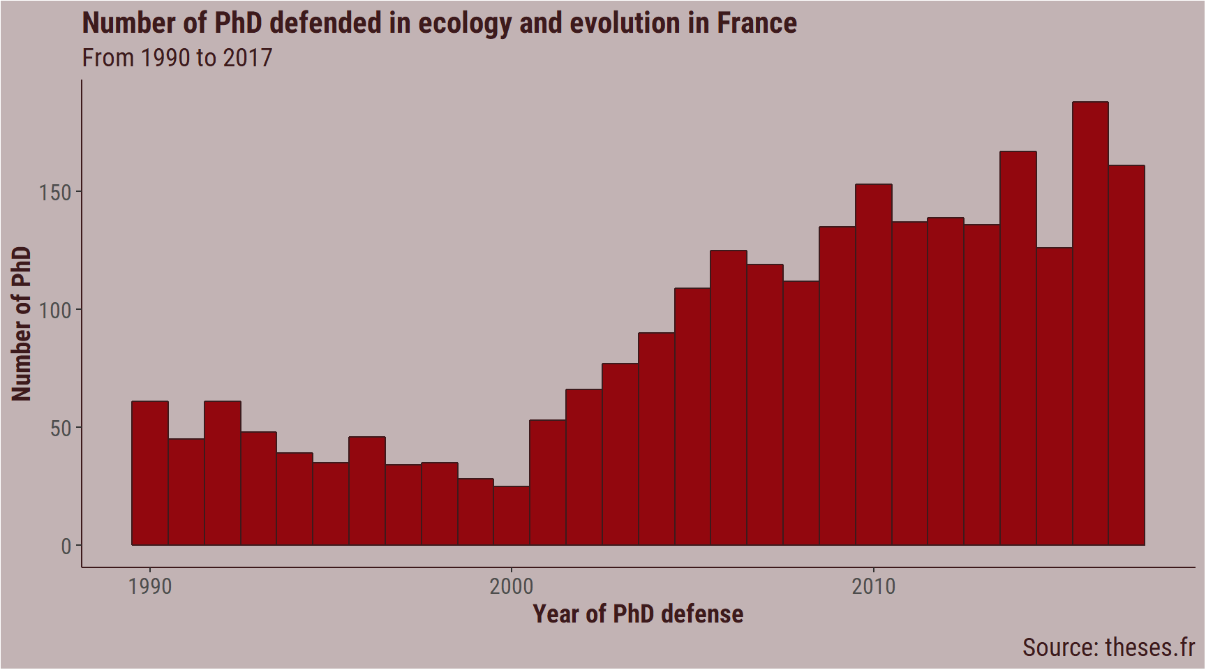
In ecology and evolution, there is also a peak of defenses in December.
thesis_evology %>%
  filter(year_defense >= 2010) %>%
    mutate(day_defense2 = day(date_defense)) %>%
  filter(day_defense2 > 1) %>%
  group_by(year_defense,
           month_defense,
           day_defense2) %>%
  count() %>%
  ggplot(aes(x = month_defense,
             y = day_defense2,
             fill = n)) +
  facet_wrap(~year_defense, ncol = 8) +
  geom_tile() +

  labs(title = "Distribution of PhD defense in ecology and evolution in France over time",
       subtitle = "",
       x = "Day of the week",
       y = "Defense month") +

scale_fill_gradient(high = bar_col,
                      low = title_colour) +

  my_theme +
  theme(axis.text.x = element_text(angle = 90,
                                   hjust = 1,
                                   vjust = 0.3))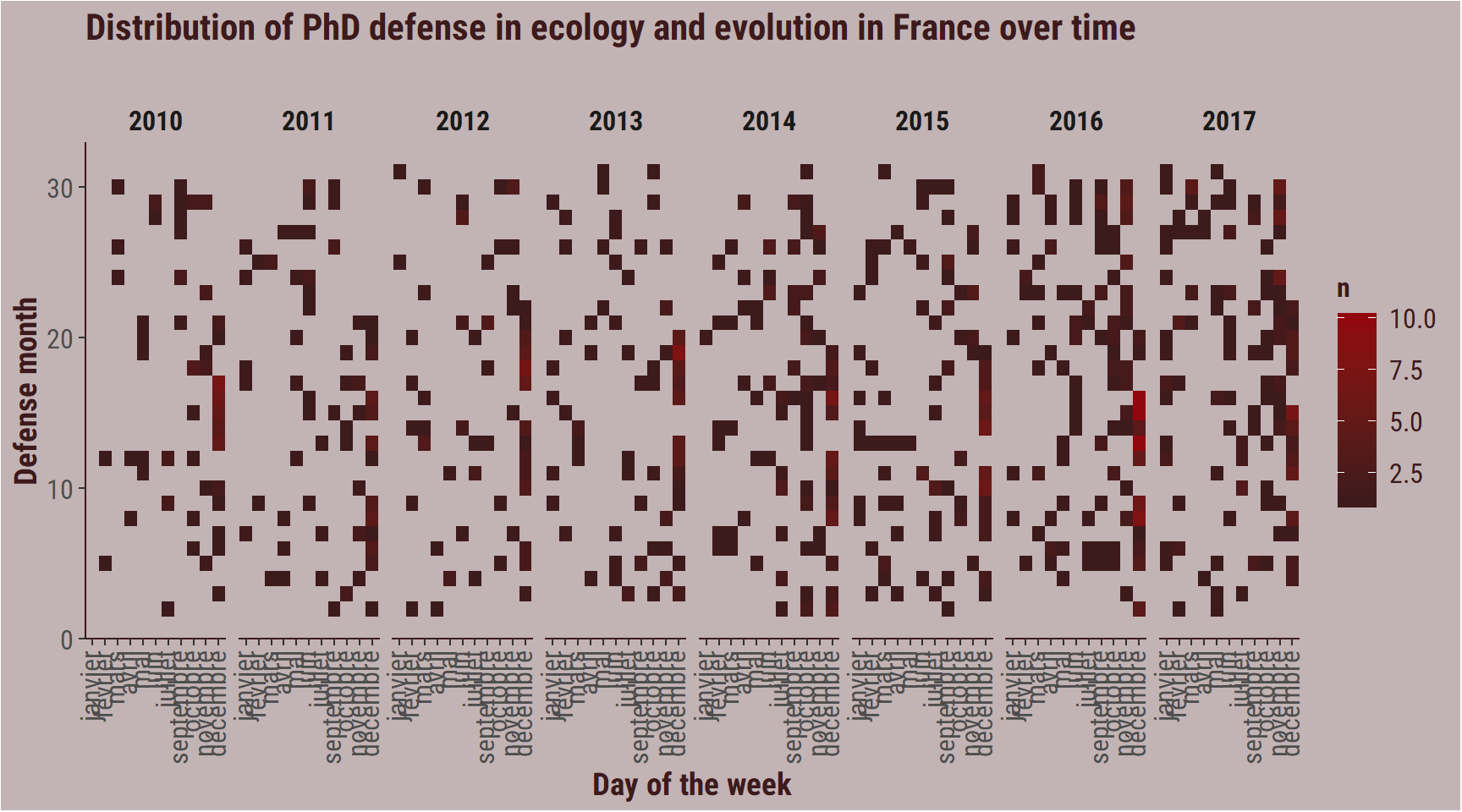
However, contrary to the general pattern, very few people defend during the week end, which corresponds to my expectations.
thesis_evology %>%
  filter(year_defense >= 2010) %>%
  mutate(day_defense2 = day(date_defense)) %>%
  filter(day_defense2 > 1) %>%
  group_by(year_defense,
           month_defense,
           day_defense) %>%
  count() %>%
  ggplot(aes(x = day_defense,
             y = month_defense,
             fill = n)) +
  facet_wrap(~year_defense, ncol = 8) +
  geom_tile() +

  labs(title = "Distribution of PhD defense in ecology and evolution in France over time",
       subtitle = "",
       x = "Day of the week",
       y = "Defense month") +

  scale_fill_gradient(high = bar_col,
                      low = title_colour) +
 my_theme +
  theme(axis.text.x = element_text(angle = 90,
                                   hjust = 1,
                                   vjust = 0.3))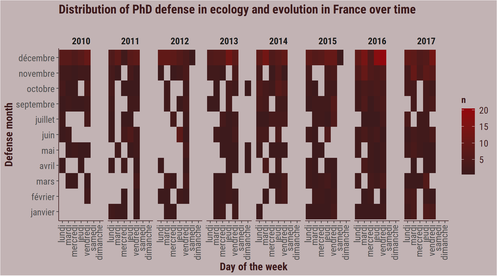
Three did, but there is nothing indicating that the date was wrong.
thesis_evology %>%
  filter(year_defense == 2013,
         day_defense == "dimanche") %>%
  select(author, date_defense) %>%
kable()| author | date_defense |
|---|---|
| Maryam Foroozanfar | 2013-05-26 |
| Azam Negahi | 2013-10-06 |
| Florent Arthaud | 2013-04-21 |